服装图像分类

​

活动地址：CSDN21天学习挑战赛

学习的最大理由是想摆脱平庸，早一天就多一份人生的精彩；迟一天就多一天平庸的困扰。各位小伙伴，如果您：
想系统/深入学习某技术知识点…
一个人摸索学习很难坚持，想组团高效学习…
想写博客但无从下手，急需写作干货注入能量…
热爱写作，愿意让自己成为更好的人…

创作计划

**
1，机缘

A，分享服装分类实验
B，日常学习中的记录
C，通过服装分类项目进行技术交流

2，收获

A，获得了10粉丝的关注
B，获得了20的赞、阅读量等
C，认识和了解了服装分类作者的想法和经验
…

3，日常

1. 创作已经是我学习的一部分了
2. 有限的时间下，利用周二、四、六进行博客创作，其余时间用来学习

4，憧憬

创作规划是学习TensorFlow图像分类方法，模型调优，使错误率减小

**

学习计划

**
1，学习目标

掌握 TensorFlow图像分类方法

2，学习内容

A，搭建TensorFlow开发环境
B，掌握 matplotlib绘图方法
C，掌握训练方法 ，损失函数的选择

3，学习时间

周一至周五晚上 7 点—晚上9点
周六下午 6点-下午 9 点
周日下午 6 点-下午 9 点

4，学习产出

技术笔记 1 遍
CSDN技术博客 10 篇
学习的vlog 视频 2 个

**

学习日记

**
1，学习知识点

服装分类方法，模型结构，数据集的结构

2，学习遇到的问题

调整数据格式、为标签编号，选择样本测试

3，学习的收获

学会了识别数据集的方式、数据可视化、使用模型预测

4，实操

import tensorflow as tf
from tensorflow.keras import datasets, layers, models
import matplotlib.pyplot as plt
import numpy as np


(train_images, train_labels), (test_images, test_labels) = datasets.fashion_mnist.load_data()
# 将像素的值标准化至0到1的区间内。
train_images, test_images = train_images / 255.0, test_images / 255.0
print(train_images.shape,test_images.shape,train_labels.shape,test_labels.shape)
#调整数据到我们需要的格式
train_images = train_images.reshape((60000, 28, 28, 1))
test_images = test_images.reshape((10000, 28, 28, 1))
print(train_images.shape,test_images.shape,train_labels.shape,test_labels.shape)

class_names = ['T-shirt/top', 'Trouser', 'Pullover', 'Dress', 'Coat',
               'Sandal', 'Shirt', 'Sneaker', 'Bag', 'Ankle boot']

 plt.figure(figsize=(20,10))
 for i in range(20):
     plt.subplot(5,4,i+1)
     plt.xticks([])
     plt.yticks([])
     plt.grid(False)
     plt.imshow(train_images[i], cmap=plt.cm.binary)
     plt.xlabel(class_names[train_labels[i]])
 plt.show()

model = models.Sequential([
    layers.Conv2D(32, (3, 3), activation='relu', input_shape=(28, 28, 1)),  # 卷积层
    layers.MaxPooling2D((2, 2)),  # 池化层
    layers.Conv2D(64, (3, 3), activation='relu'),  # 卷积层
    layers.MaxPooling2D((2, 2)),  # 池化层2，2*2采样
    layers.Conv2D(64, (3, 3), activation='relu'),  # 卷积层

    layers.Flatten(),  # Flatten层
    layers.Dense(64, activation='relu'),  # 全连接层
    layers.Dense(10)  # 输出层
])

model.summary()
model.compile(optimizer='adam',
              loss=tf.keras.losses.SparseCategoricalCrossentropy(from_logits=True),
              metrics=['accuracy'])
history = model.fit(train_images, train_labels, epochs=10,
                    validation_data=(test_images, test_labels))

acc = history.history['accuracy']
val_acc = history.history['val_accuracy']
epochs = range(1, len(acc) + 1)

plt.plot(epochs, acc, label='accuracy')
plt.plot(epochs,val_acc, label = 'val_accuracy')
plt.xlabel('Epoch')
plt.ylabel('Accuracy')
plt.ylim([0.5, 1])
plt.legend(loc='lower right')
plt.show()

test_loss, test_acc = model.evaluate(test_images,  test_labels, verbose=2)
print(test_loss,test_acc)
#测试
print('选择一个样本：',class_names[test_labels[5]])

pre = model.predict(test_images)
print('预测值：',class_names[np.argmax(pre[5])])


1
2
3
4
5
6
7
8
9
10
11
12
13
14
15
16
17
18
19
20
21
22
23
24
25
26
27
28
29
30
31
32
33
34
35
36
37
38
39
40
41
42
43
44
45
46
47
48
49
50
51
52
53
54
55
56
57
58
59
60
61
62
63
64
65
66
67
68

输出：

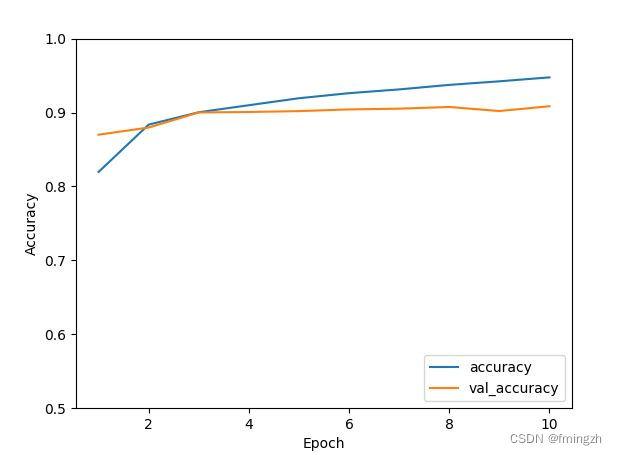
0.28127503395080566 0.9085000157356262
选择一个样本： Trouser
预测值： Trouser

分析：可以看出训练集和验证集的精确率相似，拟合效果较好。预测错误率为28%，精确率为90.6%。训练效果较好。对模型选择测试集上​的一个样本进行测试，结果正确。