【python海洋专题十七】读取几十年的OHC数据，画四季图

本期内容

读取多年数据，画四季图

Part01.

多年数据处理

图片
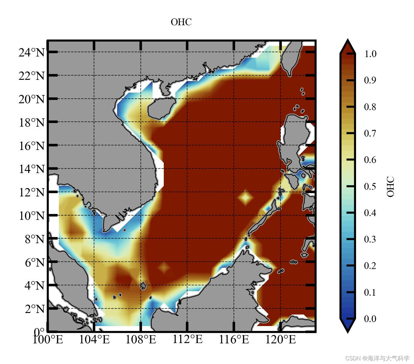
多年年平均的OHC分布

图片
春夏秋冬：

ohc_all_new = np.reshape(ohc_new, (12, 80, 29, 27), order=‘C’)
ohc_all_season_mean = np.mean(ohc_all_new, axis=1)
ohc_season = np.reshape(ohc_all_season_mean, (3, 4, 29, 27), ‘C’)
ohc_season_mean = np.mean(ohc_season, axis=0)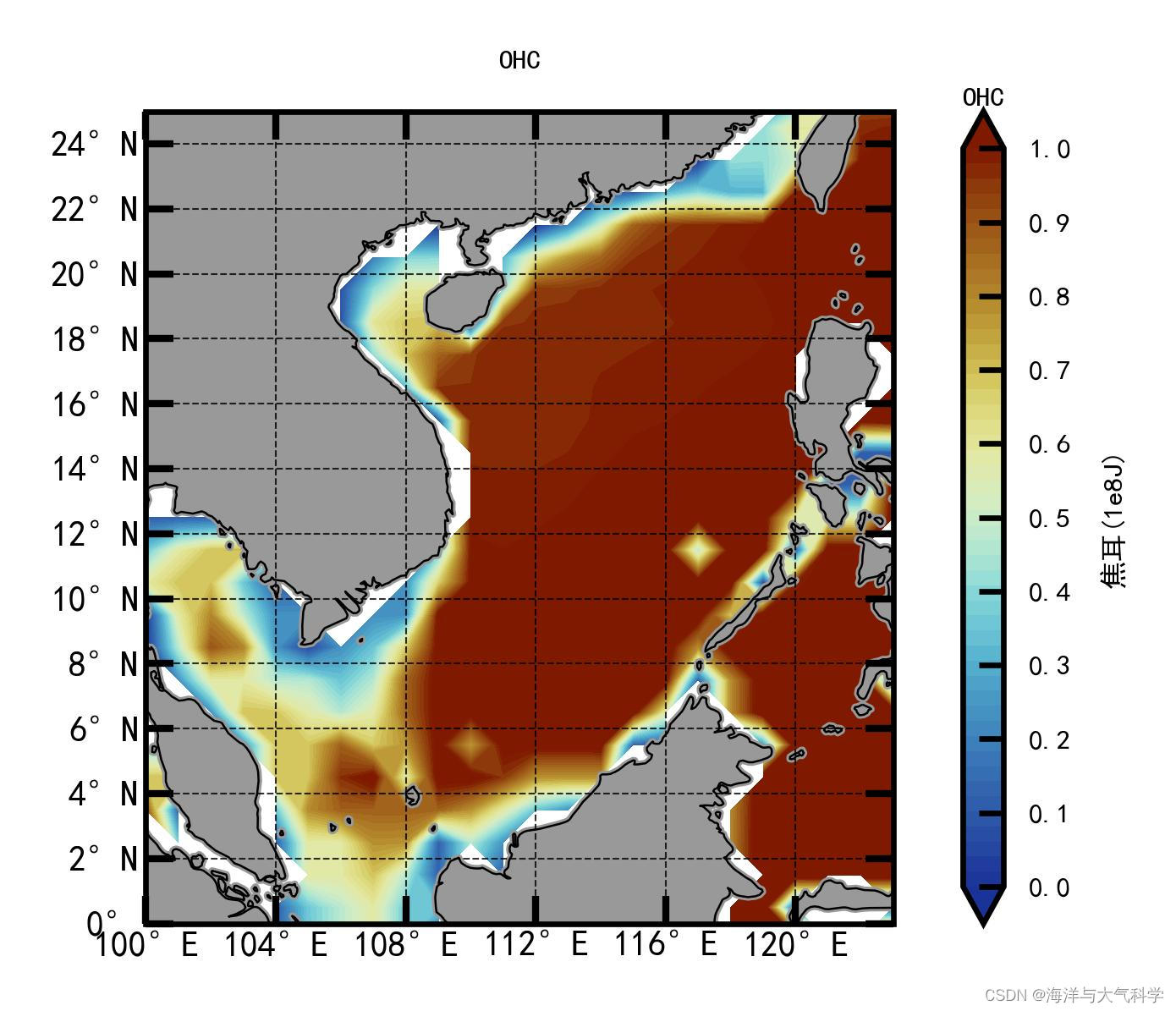

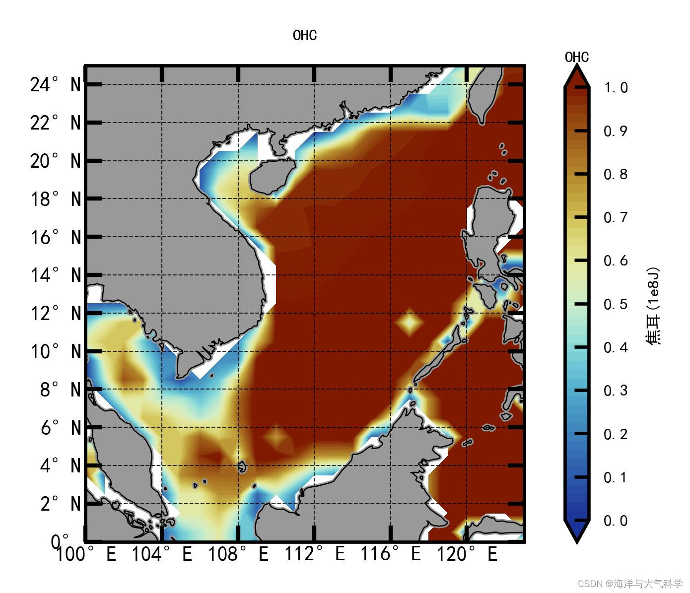
我看变化不大啊！不会数据处理问题吧！

于是又画了一年的四季：

一年的平均：

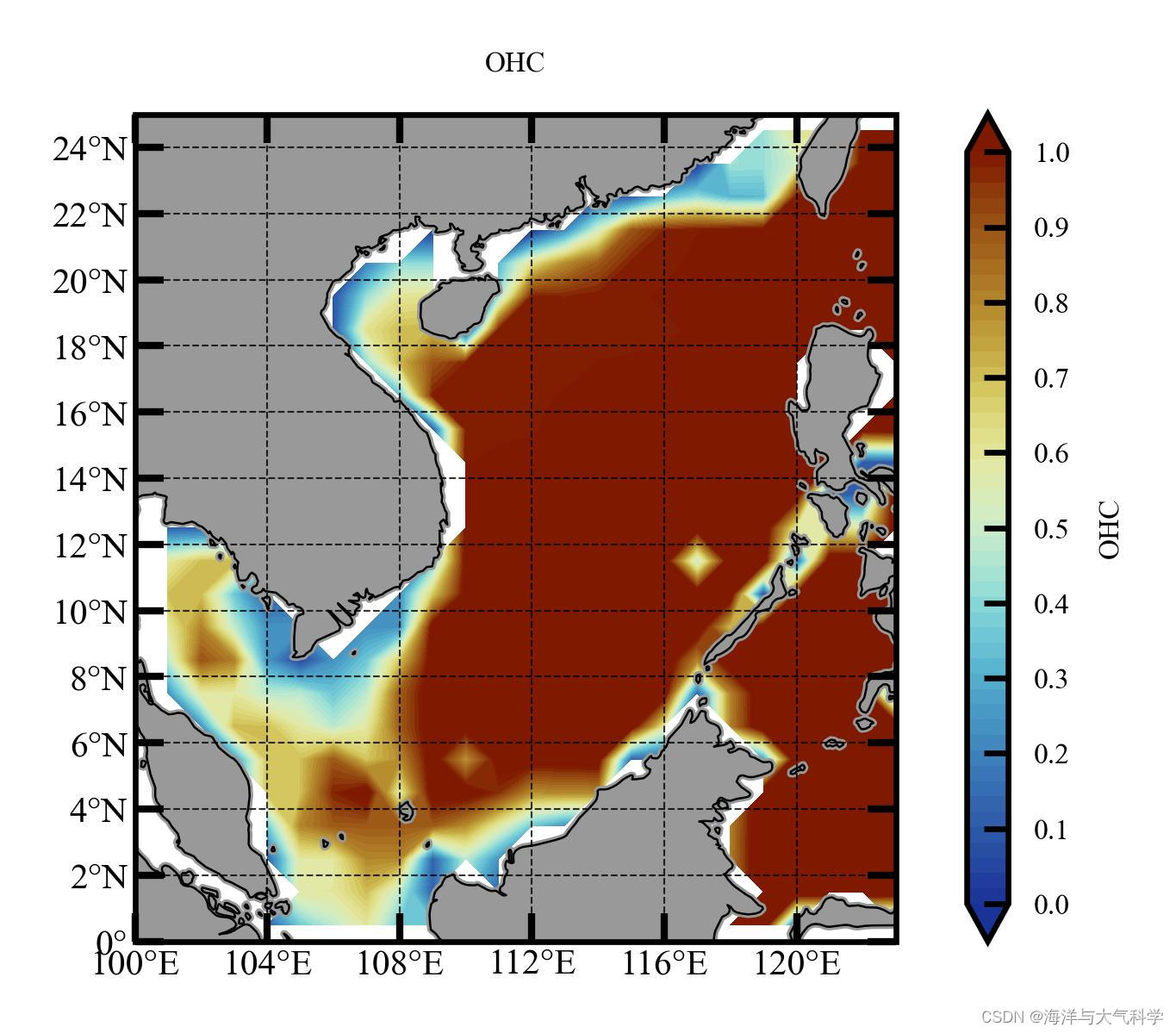
tem_spr = (tem_all[2,:,:]+tem_all[3,:,:]+tem_all[4,:,:])/3

3：sum季6-7-8

tem_sum = (tem_all[5,:,:]+tem_all[6,:,:]+tem_all[7,:,:])/3

4：aut季9-10-11

tem_aut = (tem_all[8,:,:]+tem_all[9,:,:]+tem_all[10,:,:])/3

5：win季12-1-2

tem_win = (tem_all[0,:,:]+tem_all[1,:,:]+tem_all[11,:,:])/3

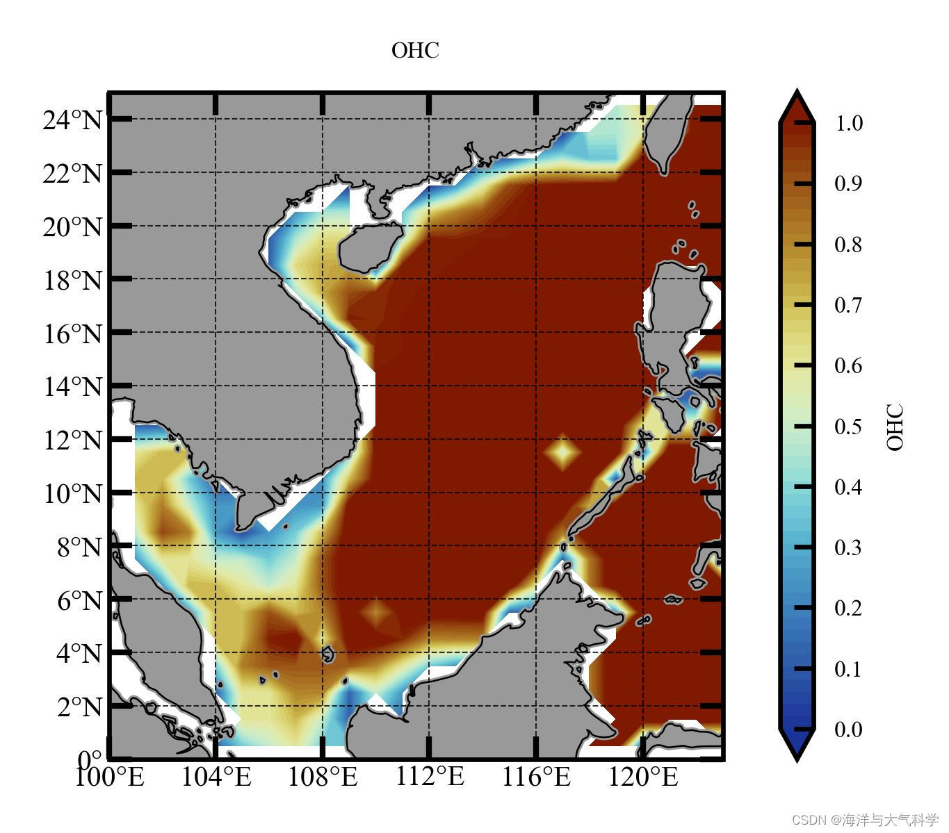
一年的四季变化也不是很大。

说明热含量一年四季变化就是不大哈！

全文代码

图片
多年的四季：一年的四季：以前更新过了哈！

# -*- coding: utf-8 -*-
# %%
# Importing related function packages
import matplotlib.pyplot as plt
import cartopy.crs as ccrs
import cartopy.feature as feature
import numpy as np
import matplotlib.ticker as ticker
from cartopy import mpl
from cartopy.mpl.ticker import LongitudeFormatter, LatitudeFormatter
from cartopy.mpl.gridliner import LONGITUDE_FORMATTER, LATITUDE_FORMATTER
from matplotlib.font_manager import FontProperties
from netCDF4 import Dataset
from pylab import *
import seaborn as sns
from matplotlib import cm
from pathlib import Path
import xarray as xr
import palettable
from palettable.cmocean.diverging import Delta_4
from palettable.colorbrewer.sequential import GnBu_9
from palettable.colorbrewer.sequential import Blues_9
from palettable.scientific.diverging import Roma_20
from palettable.cmocean.diverging import Delta_20
from palettable.scientific.diverging import Roma_20
from palettable.cmocean.diverging import Balance_20
from matplotlib.colors import ListedColormap
import pickle


# ----define reverse_colourmap----
def reverse_colourmap(cmap, name='my_cmap_r'):
    reverse = []
    k = []

    for key in cmap._segmentdata:
        k.append(key)
        channel = cmap._segmentdata[key]
        data = []

        for t in channel:
            data.append((1 - t[0], t[2], t[1]))
        reverse.append(sorted(data))

    LinearL = dict(zip(k, reverse))
    my_cmap_r = mpl.colors.LinearSegmentedColormap(name, LinearL)
    return my_cmap_r


# ---colormap----
cmap01 = Balance_20.mpl_colormap
cmap0 = Blues_9.mpl_colormap
cmap_r = reverse_colourmap(cmap0)
cmap1 = GnBu_9.mpl_colormap
cmap_r1 = reverse_colourmap(cmap1)
cmap2 = Roma_20.mpl_colormap
cmap_r2 = reverse_colourmap(cmap2)
# -------------# 指定文件路径，实现批量读取满足条件的文件------------
filepath = Path('E:\data\IAP\IAP_ocean_heat_content_data\IAP_Ocean_heat_content_0_2000m\\')
filelist = list(filepath.glob('*.nc'))
print(filelist)
# -------------读取其中一个文件的经纬度数据，制作经纬度网格（这样就不需要重复读取）-------------------------
a = Dataset(filelist[1])
print(a)
# 随便读取一个文件（一般默认需要循环读取的文件格式一致）
f1 = xr.open_dataset(filelist[1])
print(f1)
# 提取经纬度（这样就不需要重复读取）
lat = f1['lat'].data
lon = f1['lon'].data
# -------- find scs 's temp-----------
print(np.where(lon >= 100))  # 99
print(np.where(lon >= 123))  # 122
print(np.where(lat >= 0))  # 90
print(np.where(lat >= 25))  # 115
# # 画图网格
lon1 = lon[98:125]
lat1 = lat[88:117]
X, Y = np.meshgrid(lon1, lat1)
# ----------4.for循环读取文件+数据处理------------------
ohc_all = []
for file in filelist:
    with xr.open_dataset(file) as f:
        ohc = f['OHC100'].data
        ohc_mon = ohc[88:117, 98:125]
        ohc_all.append(ohc_mon)
ohc_all = np.array(ohc_all)
type(ohc_all)
print(type(ohc_all))
print(ohc_all.shape)
ohc_new = ohc_all[2:962, :, :]
print(ohc_new.shape)
ohc_all_new = np.reshape(ohc_new, (12, 80, 29, 27), order='C')
print(ohc_all_new.shape)
ohc_all_season_mean = np.mean(ohc_all_new, axis=1)
print(ohc_all_season_mean.shape)
ohc_season = np.reshape(ohc_all_season_mean, (3, 4, 29, 27), 'C')
ohc_season_mean = np.mean(ohc_season, axis=0)
print(ohc_season_mean)
ohc_all_mean = np.mean(ohc_season_mean, axis=0)
# -------------# plot  ------------
scale = '50m'
plt.rcParams['font.sans-serif'] = ['Times New Roman']  # 设置整体的字体为Times New Roman
# 设置显示中文字体
mpl.rcParams["font.sans-serif"] = ["SimHei"]
fig = plt.figure(dpi=300, figsize=(3, 2), facecolor='w', edgecolor='blue')  # 设置一个画板，将其返还给fig
ax = fig.add_axes([0.05, 0.08, 0.92, 0.8], projection=ccrs.PlateCarree(central_longitude=180))
ax.set_extent([100, 123, 0, 25], crs=ccrs.PlateCarree())  # 设置显示范围
land = feature.NaturalEarthFeature('physical', 'land', scale, edgecolor='face',
                                   facecolor=feature.COLORS['land'])
ax.add_feature(land, facecolor='0.6')
ax.add_feature(feature.COASTLINE.with_scale('50m'), lw=0.3)  # 添加海岸线：关键字lw设置线宽; lifestyle设置线型
cs = ax.contourf(X, Y, ohc_all_mean/1e10, levels=np.linspace(0, 1, 50), extend='both', cmap=cmap_r2,
                 transform=ccrs.PlateCarree())
# ------color-bar设置------------
cb = plt.colorbar(cs, ax=ax, extend='both', orientation='vertical', ticks=np.linspace(0, 1, 11))
cb.set_label('焦耳(1e8J)', fontsize=4, color='k')  # 设置color-bar的标签字体及其大小
cb.ax.set_title('OHC', fontsize=4, color='k')
cb.ax.tick_params(labelsize=4, direction='in')  # 设置color-bar刻度字体大小。
# cf = ax.contour(x, y, skt1[:, :], levels=np.linspace(16, 30, 5), colors='gray', linestyles='-',
#                 linewidths=0.2, transform=ccrs.PlateCarree())
# --------------图片 添加标题----------------
ax.set_title('OHC', fontsize=4)
# ------------------利用Formatter格式化刻度标签-----------------
ax.set_xticks(np.arange(100, 123, 4), crs=ccrs.PlateCarree())  # 添加经纬度
ax.set_xticklabels(np.arange(100, 123, 4), fontsize=4)
ax.set_yticks(np.arange(0, 25, 2), crs=ccrs.PlateCarree())
ax.set_yticklabels(np.arange(0, 25, 2), fontsize=4)
ax.xaxis.set_major_formatter(LongitudeFormatter())
ax.yaxis.set_major_formatter(LatitudeFormatter())
ax.tick_params(axis='x', top=True, which='major', direction='in', length=4, width=1, labelsize=5, pad=1, color='k')  # 刻度样式
ax.tick_params(axis='y', right=True, which='major', direction='in', length=4, width=1, labelsize=5, pad=1, color='k')  # 更改刻度指向为朝内，颜色设置为蓝色
gl = ax.gridlines(crs=ccrs.PlateCarree(), draw_labels=False, xlocs=np.arange(100, 123, 4), ylocs=np.arange(0, 25, 2),
                  linewidth=0.25, linestyle='--', color='k', alpha=0.8)  # 添加网格线
gl.top_labels, gl.bottom_labels, gl.right_labels, gl.left_labels = False, False, False, False
plt.savefig('ohc_multi_year_mean.jpg', dpi=600, bbox_inches='tight', pad_inches=0.1)  # 输出地图，并设置边框空白紧密
plt.show()
# -plot----
# -------------# plot  ------------
scale = '50m'
plt.rcParams['font.sans-serif'] = ['Times New Roman']  # 设置整体的字体为Times New Roman
# 设置显示中文字体
mpl.rcParams["font.sans-serif"] = ["SimHei"]
fig = plt.figure(dpi=300, figsize=(3, 2), facecolor='w', edgecolor='blue')  # 设置一个画板，将其返还给fig
ax = fig.add_axes([0.05, 0.08, 0.92, 0.8], projection=ccrs.PlateCarree(central_longitude=180))
ax.set_extent([100, 123, 0, 25], crs=ccrs.PlateCarree())  # 设置显示范围
land = feature.NaturalEarthFeature('physical', 'land', scale, edgecolor='face',
                                   facecolor=feature.COLORS['land'])
ax.add_feature(land, facecolor='0.6')
ax.add_feature(feature.COASTLINE.with_scale('50m'), lw=0.3)  # 添加海岸线：关键字lw设置线宽; lifestyle设置线型
cs = ax.contourf(X, Y, ohc_season_mean[0,:,:]/1e10, levels=np.linspace(0, 1, 50), extend='both', cmap=cmap_r2,
                 transform=ccrs.PlateCarree())
# ------color-bar设置------------
cb = plt.colorbar(cs, ax=ax, extend='both', orientation='vertical', ticks=np.linspace(0, 1, 11))
cb.set_label('焦耳(1e8J)', fontsize=4, color='k')  # 设置color-bar的标签字体及其大小
cb.ax.set_title('OHC', fontsize=4, color='k')
cb.ax.tick_params(labelsize=4, direction='in')  # 设置color-bar刻度字体大小。
# cf = ax.contour(x, y, skt1[:, :], levels=np.linspace(16, 30, 5), colors='gray', linestyles='-',
#                 linewidths=0.2, transform=ccrs.PlateCarree())
# --------------图片 添加标题----------------
ax.set_title('OHC', fontsize=4)
# ------------------利用Formatter格式化刻度标签-----------------
ax.set_xticks(np.arange(100, 123, 4), crs=ccrs.PlateCarree())  # 添加经纬度
ax.set_xticklabels(np.arange(100, 123, 4), fontsize=4)
ax.set_yticks(np.arange(0, 25, 2), crs=ccrs.PlateCarree())
ax.set_yticklabels(np.arange(0, 25, 2), fontsize=4)
ax.xaxis.set_major_formatter(LongitudeFormatter())
ax.yaxis.set_major_formatter(LatitudeFormatter())
ax.tick_params(axis='x', top=True, which='major', direction='in', length=4, width=1, labelsize=5, pad=1, color='k')  # 刻度样式
ax.tick_params(axis='y', right=True, which='major', direction='in', length=4, width=1, labelsize=5, pad=1, color='k')  # 更改刻度指向为朝内，颜色设置为蓝色
gl = ax.gridlines(crs=ccrs.PlateCarree(), draw_labels=False, xlocs=np.arange(100, 123, 4), ylocs=np.arange(0, 25, 2),
                  linewidth=0.25, linestyle='--', color='k', alpha=0.8)  # 添加网格线
gl.top_labels, gl.bottom_labels, gl.right_labels, gl.left_labels = False, False, False, False
plt.savefig('ohc_multi_year_spr.jpg', dpi=600, bbox_inches='tight', pad_inches=0.1)  # 输出地图，并设置边框空白紧密
plt.show()

图片
E

N

D
1
2
3
4
5
6
7
8
9
10
11
12
13
14
15
16
17
18
19
20
21
22
23
24
25
26
27
28
29
30
31
32
33
34
35
36
37
38
39
40
41
42
43
44
45
46
47
48
49
50
51
52
53
54
55
56
57
58
59
60
61
62
63
64
65
66
67
68
69
70
71
72
73
74
75
76
77
78
79
80
81
82
83
84
85
86
87
88
89
90
91
92
93
94
95
96
97
98
99
100
101
102
103
104
105
106
107
108
109
110
111
112
113
114
115
116
117
118
119
120
121
122
123
124
125
126
127
128
129
130
131
132
133
134
135
136
137
138
139
140
141
142
143
144
145
146
147
148
149
150
151
152
153
154
155
156
157
158
159
160
161
162
163
164
165
166
167
168
169
170
171
172
173
174
175
176
177
178
179
180
181
182