-
机器学习(监督学习)笔记
目录
- 总览
- 笔记内容
- 代码部分
- 实验一代码(批梯度,小批度,随机批度下降手撸)
- 实验二 线性回归代码手撸(批梯度)
- 实验三 线性回归代码手撸(随机批度)
- 实验四 线性回归代码手撸(小批度)
- 实验五 特征缩放手撸(标准化,归一化)
- 实验八 线性回归二分类
- 实验九 均方差(MSE)-逻辑回归模型
- 实验九 均方差(MSE)-逻辑回归模型3D版本
- 实验十 交叉熵-逻辑回归模型(R,P,F1)
- 实验十一 scikit-learn SVM
- 实验十二 SVM(错误率随C值变化)
- 实验十三 K交叉验证-SVM
- 实验十四 K近邻(K变化)-K交叉验证
- 实验十五 宏F1值,马修斯相关系数
- 实验十六 高斯朴素贝叶斯分类器
- 实验十七 多分类逻辑回归
- 二分类逻辑回归的不足
- 二分类逻辑回归强化
- 实验十八 二分类神经网络
- 实验十九 多分类神经网络
- 资源地址
- 总结
总览
分享一个GPU服务器租赁平台(价格十分优惠,有4090,3090,A6000等)
本文是机器学习的学习笔记(监督学习部分),全手撸了课程这部分的代码。
教材是《机器学习原理与实践》微课版,作者陈喆。笔记内容
线性回归

梯度下降


特征缩放

多输出线性回归


逻辑回归
二分类与逻辑回归


分类任务的性能指标(召回率,精度,F1分数等)


支持向量机SVM


K近邻


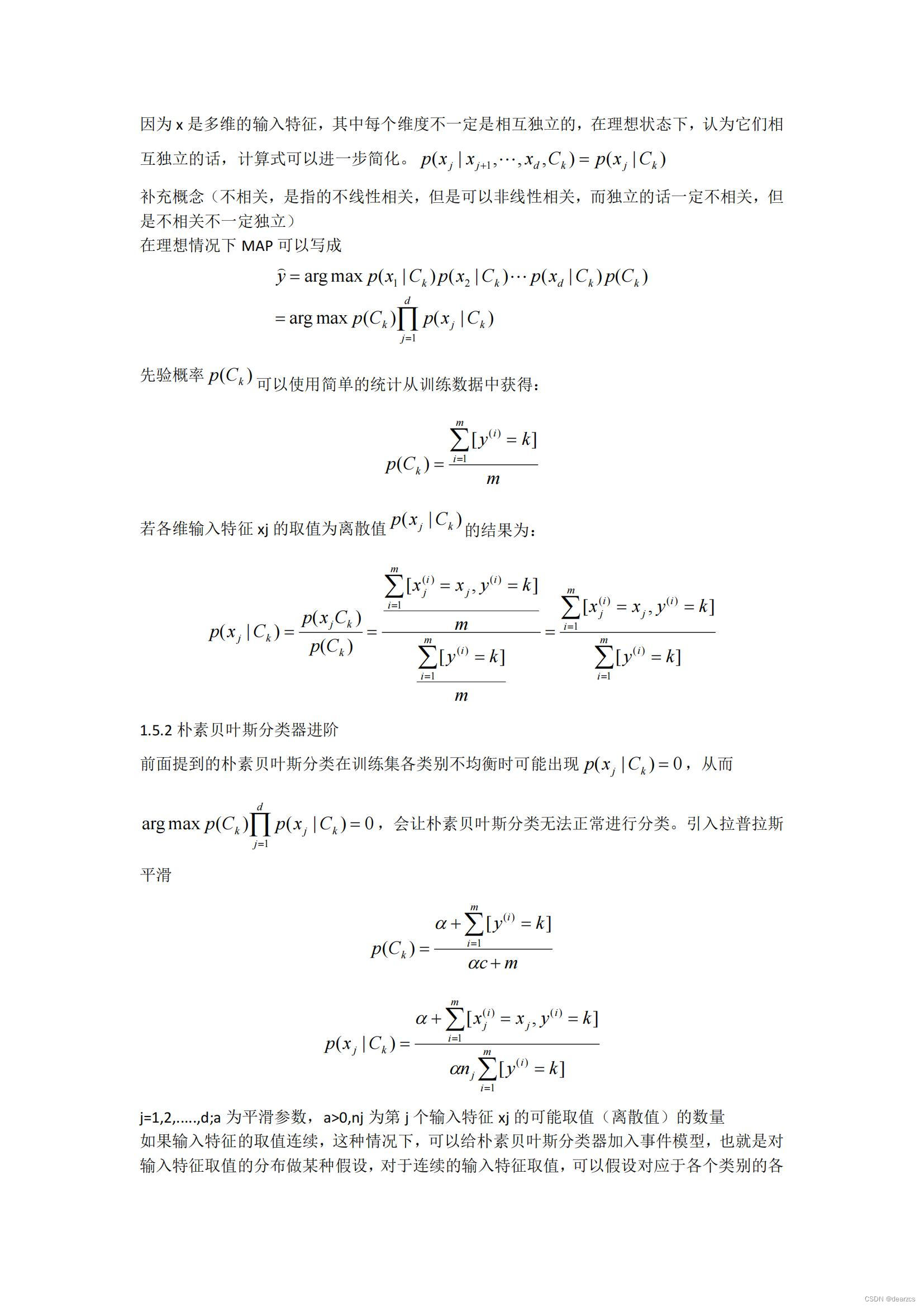
朴素贝叶斯分类器

朴素贝叶斯分类器进阶


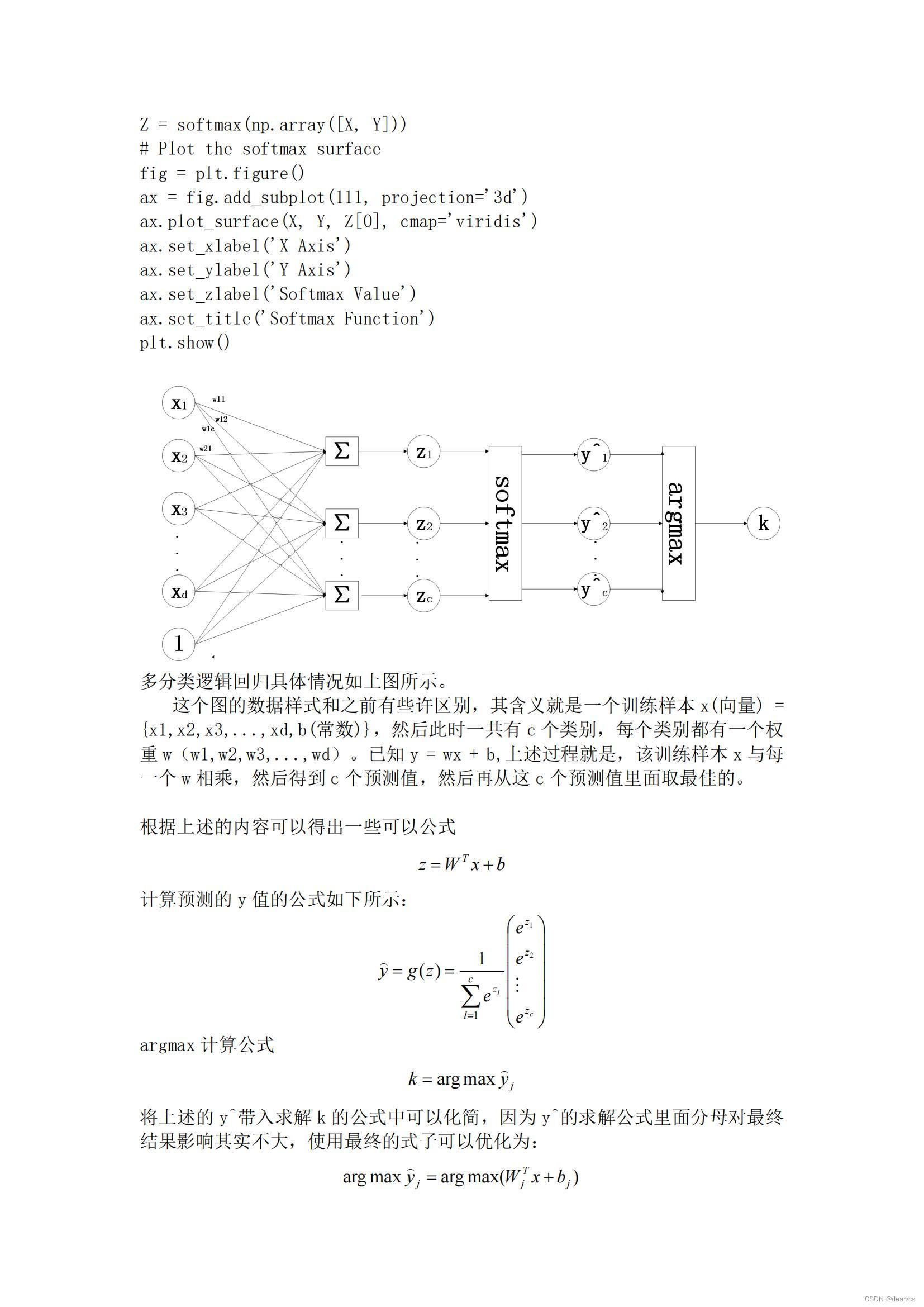
多分类逻辑回归


二分类神经网络


多分类神经网络


代码部分
实验一代码(批梯度,小批度,随机批度下降手撸)
# 实验2-1 # 批梯度下降 import pandas as pd import numpy as np import random as rd import matplotlib.pyplot as plt # load dataset df = pd.read_csv('temperature_dataset.csv') data = np.array(df) y0 = np.array([i[0] for i in data]) # 第一列作为样本标注 y14 = np.array([i[1:] for i in data])#2-5 作为四维输出特征 xuexi = 0.0001 # 学习率 ep = 20 epoch = [ep] # 遍历次数 m = np.size(data,0) # 获取样本长度 m alls = [i for i in range(m)] trainsyo = [] # 训练集标注 testyo = [] # 测试集标注 trainsy14 = [] # 训练集输入特征 testy14 = [] # 测试集输入特征 tra = int(m * 0.8) # 训练集长度 tes = m - tra # 测试集长度 for i in range(tra): # 获取训练集 a = rd.choice(alls) # 从alls中随机选取一个 trainsyo.append(y0[a]) # 增加训练集标注 trainsy14.append(y14[a])# 增加训练集输入特征 alls.remove(a) trainsy14 = np.array(trainsy14) # 训练集list转变array trainsyo = np.array(trainsyo) # 训练集list转变array for a in alls: # 获取测试集 # global y0 # global y14 testyo.append(y0[a])# 增加测试集标注 testy14.append(y14[a]) # 增加测试集输入特征 w = np.array([rd.random() for i in range(4)]) # 初次随机获取权重w # print(w) b = [rd.random()] # 初次随机获取偏差b RMSE = [] # 均方根误差 RMSE2 = [] # 训练集 while(epoch[0]): # 开始遍历 epoch[0] -= 1 # 设置的超参数epoch -1 e =np.dot(testy14,w.transpose()) + b[0] - testyo RMSE.append((np.dot(e,e.transpose())/tes)**0.5) e = np.dot(trainsy14,w.transpose()) + b[0] - trainsyo # n*1 RMSE2.append((np.dot(e,e.transpose())/tra)**0.5) b[0] -= 2*xuexi*np.dot(np.ones(tra),e)/tra w -= 2*xuexi*np.dot(e.transpose(),trainsy14)/tra # 绘图部分 plt.rcParams['font.sans-serif']=['SimHei'] #用来正常显示中文标签 plt.rcParams['axes.unicode_minus']=False #用来正常显示负号 x = [i+1 for i in range(ep)] # 设置x坐标 print(min(RMSE),min(RMSE2)) ymax = max(RMSE) + 1 plt.xlabel('epoch') # 设置x坐标名称 plt.ylabel('RMSE') # 设置y坐标名称 plt.title('训练情况') # 设置标题 plt.plot(x,RMSE,color='r',marker='o',linestyle='dashed') # plt.plot(x,RMSE,color='r') # 设置绘图的基本参数 plt.axis([0,ep+ 1,0,ymax]) # 设置xy的取值范围 plt.show() # 展示图片- 1
- 2
- 3
- 4
- 5
- 6
- 7
- 8
- 9
- 10
- 11
- 12
- 13
- 14
- 15
- 16
- 17
- 18
- 19
- 20
- 21
- 22
- 23
- 24
- 25
- 26
- 27
- 28
- 29
- 30
- 31
- 32
- 33
- 34
- 35
- 36
- 37
- 38
- 39
- 40
- 41
- 42
- 43
- 44
- 45
- 46
- 47
- 48
- 49
- 50
- 51
- 52
- 53
- 54
- 55
- 56
- 57
- 58
- 59
- 60
- 61
实验二 线性回归代码手撸(批梯度)
# 2-2 import pandas as pd import numpy as np import random as rd import matplotlib.pyplot as plt # load dataset df = pd.read_csv('temperature_dataset.csv') data = np.array(df) y0 = np.array([i[0] for i in data]) # 第一列作为样本标注 y14 = np.array([i[3] for i in data])# 选第三维作为输入特征 xuexi = 0.0001 # 学习率 ep = 20 epoch = [ep] # 遍历次数 m = np.size(data,0) # 获取样本长度 m alls = [i for i in range(m)] trainsyo = [] # 训练集标注 testyo = [] # 测试集标注 trainsy14 = [] # 训练集输入特征 testy14 = [] # 测试集输入特征 tra = int(m * 0.8) # 训练集长度 tes = m - tra # 测试集长度 allw = [] # 训练过程中的全部的w allb = [] # 训练过程中的全部的b for i in range(tra): # 获取训练集 a = rd.choice(alls) # 从alls中随机选取一个 trainsyo.append(y0[a]) # 增加训练集标注 trainsy14.append(y14[a])# 增加训练集输入特征 alls.remove(a) trainsy14 = np.array(trainsy14) # 训练集list转变array trainsyo = np.array(trainsyo) # 训练集list转变array for a in alls: # 获取测试集 # global y0 # global y14 testyo.append(y0[a])# 增加测试集标注 testy14.append(y14[a]) # 增加测试集输入特征 w = np.array([rd.random() for i in range(1)]) # 初次随机获取权重w # print(w) b = [rd.random()] # 初次随机获取偏差b RMSE = [] # 均方根误差 while(epoch[0]): # 开始遍历 epoch[0] -= 1 # 设置的超参数epoch -1 newb = 0 # 求解的b的值 newW = int() # 求解的w的值 for i in range(tra): # 遍历全部的训练集 a = np.dot(w,trainsy14[i].transpose()) + b[0] - trainsyo[i] # 计算(W*xT + b - y ) newb += float(a) # 累加 if type(newW) == int: newW = trainsy14[i].transpose()*float(a) # 初次赋值 else: newW += trainsy14[i].transpose()*float(a) # 累加w w -= xuexi*newW * (2/tra) # 更新w b[0] -= xuexi*newb *2 / tra # 更新b allw.append(w[0]) allb.append(b[0]) yall = [] xs= [-5,-3,--1,0,1,3,5] # x 轴模板 xall = [xs for i in range(ep)] ymax = 0 ymin = 30 for i in range(ep): yall.append([allw[i]*t + allb[i] for t in xs]) ymax = max(ymax,max(yall[i])) ymin = min(ymin,min(yall[i])) #绘图部分 plt.rcParams['font.sans-serif']=['SimHei'] #用来正常显示中文标签 plt.rcParams['axes.unicode_minus']=False #用来正常显示负号 x = [i+1 for i in range(ep)] # 设置x坐标 plt.xlabel('x') # 设置x坐标名称 plt.ylabel('y') # 设置y坐标名称 plt.title('拟合直线变化') # 设置标题 plots = [] for i in range(ep): c='r' if i == 0: c = 'b' elif i == ep -1: c = 'k' p, = plt.plot(xall[i],yall[i],color=c,marker='o',linestyle='dashed') plots.append(p) # plt.plot(x,RMSE,color='r') # 设置绘图的基本参数 plt.legend((plots[0],plots[-1]),['start','end']) plt.axis([-6,6,ymin-1,ymax+1]) # 设置xy的取值范围 plt.show() # 展示图片- 1
- 2
- 3
- 4
- 5
- 6
- 7
- 8
- 9
- 10
- 11
- 12
- 13
- 14
- 15
- 16
- 17
- 18
- 19
- 20
- 21
- 22
- 23
- 24
- 25
- 26
- 27
- 28
- 29
- 30
- 31
- 32
- 33
- 34
- 35
- 36
- 37
- 38
- 39
- 40
- 41
- 42
- 43
- 44
- 45
- 46
- 47
- 48
- 49
- 50
- 51
- 52
- 53
- 54
- 55
- 56
- 57
- 58
- 59
- 60
- 61
- 62
- 63
- 64
- 65
- 66
- 67
- 68
- 69
- 70
- 71
- 72
- 73
- 74
- 75
- 76
- 77
- 78
- 79
- 80
- 81
- 82
- 83
实验三 线性回归代码手撸(随机批度)
# 2-3 # 随机梯度下降 import pandas as pd import numpy as np import random as rd import matplotlib.pyplot as plt # load dataset np.random.seed(100) rng = np.random.default_rng() df = pd.read_csv('temperature_dataset.csv') data = np.array(df) y0 = np.array([i[0] for i in data]) # 第一列作为样本标注 y14 = np.array([i[1:] for i in data])#2-5 作为四维输出特征 xuexi = 0.0001 # 学习率 ep = 200 epoch = [ep] # 遍历次数 m = np.size(data,0) # 获取样本长度 m alls = [i for i in range(m)] trainsyo = [] # 训练集标注 testyo = [] # 测试集标注 trainsy14 = [] # 训练集输入特征 testy14 = [] # 测试集输入特征 tra = int(m * 0.8) # 训练集长度 tes = m - tra # 测试集长度 for i in range(tra): # 获取训练集 a = rd.choice(alls) # 从alls中随机选取一个 trainsyo.append(y0[a]) # 增加训练集标注 trainsy14.append(y14[a])# 增加训练集输入特征 alls.remove(a) trainsy14 = np.array(trainsy14) # 训练集list转变array trainsyo = np.array(trainsyo) # 训练集list转变array for a in alls: # 获取测试集 # global y0 # global y14 testyo.append(y0[a])# 增加测试集标注 testy14.append(y14[a]) # 增加测试集输入特征 w = np.array([rd.random() for i in range(4)]) # 初次随机获取权重w # print(w) b = [rd.random()] # 初次随机获取偏差b RMSE = [] # 均方根误差 while(epoch[0]): # 开始遍历 epoch[0] -= 1 # 设置的超参数epoch -1 newtra = [i for i in range(tra)] rd.shuffle(newtra) i = rd.choice(newtra) a = np.dot(w,trainsy14[i].transpose()) + b[0] - trainsyo[i] # 计算(W*xT + b - y ) b[0] -= 2*xuexi*a w -= 2*xuexi*trainsy14[i].transpose()*a # 初次赋值 y = 0 # 中间变量用于存储RMSE每一轮的 for i in range(tes): # y += (np.dot(w,testy14[i].transpose()) + b[0] - testyo[i])**2 # 计算均方根误差,并累加 RMSE.append((y/tes)**0.5) # 绘图部分 plt.rcParams['font.sans-serif']=['SimHei'] #用来正常显示中文标签 plt.rcParams['axes.unicode_minus']=False #用来正常显示负号 x = [i+1 for i in range(ep)] # 设置x坐标 print(min(RMSE)) ymax = max(RMSE) + 1 plt.xlabel('epoch') # 设置x坐标名称 plt.ylabel('RMSE') # 设置y坐标名称 plt.title('训练情况') # 设置标题 plt.plot(x,RMSE,color='r',marker='o',linestyle='dashed') # plt.plot(x,RMSE,color='r') # 设置绘图的基本参数 plt.axis([0,ep+ 1,0,ymax]) # 设置xy的取值范围 plt.show() # 展示图片- 1
- 2
- 3
- 4
- 5
- 6
- 7
- 8
- 9
- 10
- 11
- 12
- 13
- 14
- 15
- 16
- 17
- 18
- 19
- 20
- 21
- 22
- 23
- 24
- 25
- 26
- 27
- 28
- 29
- 30
- 31
- 32
- 33
- 34
- 35
- 36
- 37
- 38
- 39
- 40
- 41
- 42
- 43
- 44
- 45
- 46
- 47
- 48
- 49
- 50
- 51
- 52
- 53
- 54
- 55
- 56
- 57
- 58
- 59
- 60
- 61
- 62
- 63
- 64
- 65
- 66
- 67
实验四 线性回归代码手撸(小批度)
# 2-4 # 小批梯度下降 import pandas as pd import numpy as np import random as rd import matplotlib.pyplot as plt # load dataset df = pd.read_csv('temperature_dataset.csv') data = np.array(df) y0 = np.array([i[0] for i in data]) # 第一列作为样本标注 y14 = np.array([i[1:] for i in data])#2-5 作为四维输出特征 xuexi = 0.0001 # 学习率 batch = 30 # 设置批长度 ep = 20 # 设置遍历次数 epoch = [ep] # 遍历次数 m = np.size(data,0) # 获取样本长度 m alls = [i for i in range(m)] trainsyo = [] # 训练集标注 testyo = [] # 测试集标注 trainsy14 = [] # 训练集输入特征 testy14 = [] # 测试集输入特征 tra = int(m * 0.8) # 训练集长度 tes = m - tra # 测试集长度 for i in range(tra): # 获取训练集 a = rd.choice(alls) # 从alls中随机选取一个 trainsyo.append(y0[a]) # 增加训练集标注 trainsy14.append(y14[a])# 增加训练集输入特征 alls.remove(a) trainsy14 = np.array(trainsy14) # 训练集list转变array trainsyo = np.array(trainsyo) # 训练集list转变array for a in alls: # 获取测试集 # global y0 # global y14 testyo.append(y0[a])# 增加测试集标注 testy14.append(y14[a]) # 增加测试集输入特征 w = np.array([rd.random() for i in range(4)]) # 初次随机获取权重w # print(w) b = [rd.random()] # 初次随机获取偏差b RMSE2 = [] RMSE = [] # 均方根误差 while(epoch[0]): # 开始遍历 epoch[0] -= 1 # 设置的超参数epoch -1 if not batch:break times = tra // batch if tra % batch: times += 1 for _ in range(times): starts = _*batch ends = (_+1)*batch if (_+1)*batch >= tra: ends = tra batch = tra%batch if(not batch):break e =np.dot(testy14,w.transpose()) + b[0] - testyo RMSE.append((np.dot(e,e.transpose())/tes)**0.5) e = np.dot(trainsy14[starts:ends],w.transpose()) + b[0] - trainsyo[starts:ends] # n*1 RMSE2.append((np.dot(e,e.transpose())/batch)**0.5) b[0] -= 2*xuexi*np.dot(np.ones(batch),e)/batch w -= 2*xuexi*np.dot(e.transpose(),trainsy14[starts:ends])/batch # 绘图部分 print(min(RMSE)) plt.rcParams['font.sans-serif']=['SimHei'] #用来正常显示中文标签 plt.rcParams['axes.unicode_minus']=False #用来正常显示负号 x = [i+1 for i in range(20)] # 设置x坐标 RMSE = RMSE[:20] ymax = max(RMSE[:20]) + 1 plt.xlabel('epoch') # 设置x坐标名称 plt.ylabel('RMSE') # 设置y坐标名称 plt.title('训练情况') # 设置标题 plt.plot(x,RMSE,color='r',marker='o',linestyle='dashed') # plt.plot(x,RMSE,color='r') # 设置绘图的基本参数 plt.axis([-2,len(RMSE)+ 6,0,ymax+3]) # 设置xy的取值范围 plt.show() # 展示图片- 1
- 2
- 3
- 4
- 5
- 6
- 7
- 8
- 9
- 10
- 11
- 12
- 13
- 14
- 15
- 16
- 17
- 18
- 19
- 20
- 21
- 22
- 23
- 24
- 25
- 26
- 27
- 28
- 29
- 30
- 31
- 32
- 33
- 34
- 35
- 36
- 37
- 38
- 39
- 40
- 41
- 42
- 43
- 44
- 45
- 46
- 47
- 48
- 49
- 50
- 51
- 52
- 53
- 54
- 55
- 56
- 57
- 58
- 59
- 60
- 61
- 62
- 63
- 64
- 65
- 66
- 67
- 68
- 69
- 70
- 71
- 72
- 73
实验五 特征缩放手撸(标准化,归一化)
#2-5 # 各种标准化 import pandas as pd import numpy as np import random as rd import matplotlib.pyplot as plt # load dataset df = pd.read_csv('temperature_dataset.csv') data = np.array(df) y0 = np.array([i[0] for i in data]) # 第一列作为样本标注 y14 = np.array([i[1:] for i in data])#2-5 作为四维输出特征 # 标准化 # mean = np.mean(y14,0) # 平均值 # stds = np.std(y14,0,ddof=1) # y14 = (y14-mean)/stds # 最小最大归一化 # maxs = np.amax(y14,0) # mins = np.amin(y14,0) # y14 = (y14 - mins)/(maxs-mins) # 均值归一化 mean = np.mean(y14,0) # 平均值 maxs = np.amax(y14,0) mins = np.amin(y14,0) y14 = (y14-mean)/(maxs - mins) xuexi = 0.1 # 学习率 ep = 2000 epoch = [ep] # 遍历次数 m = np.size(data,0) # 获取样本长度 m alls = [i for i in range(m)] trainsyo = [] # 训练集标注 testyo = [] # 测试集标注 trainsy14 = [] # 训练集输入特征 testy14 = [] # 测试集输入特征 tra = int(m * 0.8) # 训练集长度 tes = m - tra # 测试集长度 for i in range(tra): # 获取训练集 a = rd.choice(alls) # 从alls中随机选取一个 trainsyo.append(y0[a]) # 增加训练集标注 trainsy14.append(y14[a])# 增加训练集输入特征 alls.remove(a) trainsy14 = np.array(trainsy14) # 训练集list转变array trainsyo = np.array(trainsyo) # 训练集list转变array for a in alls: # 获取测试集 testyo.append(y0[a])# 增加测试集标注 testy14.append(y14[a]) # 增加测试集输入特征 # w = np.array([rd.random() for i in range(4)]) # 初次随机获取权重w w =np.array([0.,0.,0.,0.]) # print(w) # b = [rd.random()] # 初次随机获取偏差b b = [0.] RMSE = [] # 均方根误差 RMSE2 = [] # 训练集均方根误差 while(epoch[0]): # 开始遍历 epoch[0] -= 1 # 设置的超参数epoch -1 e =np.dot(testy14,w.transpose()) + b[0] - testyo RMSE.append((np.dot(e,e.transpose())/tes)**0.5) e = np.dot(trainsy14,w.transpose()) + b[0] - trainsyo # n*1 RMSE2.append((np.dot(e,e.transpose())/tra)**0.5) b[0] -= 2*xuexi*np.dot(np.ones(tra),e)/tra w -= 2*xuexi*np.dot(e.transpose(),trainsy14)/tra # 绘图部分 plt.rcParams['font.sans-serif']=['SimHei'] #用来正常显示中文标签 plt.rcParams['axes.unicode_minus']=False #用来正常显示负号 x = [i+1 for i in range(ep)] # 设置x坐标 print(min(RMSE),min(RMSE2)) ymax = max(RMSE) + 1 plt.xlabel('epoch') # 设置x坐标名称 plt.ylabel('RMSE') # 设置y坐标名称 plt.title('训练情况') # 设置标题 plt.plot(x,RMSE,color='r',linestyle='dashed') plt.plot(x,RMSE2,color='k',linestyle='dashed') # plt.plot(x,RMSE,color='r') # 设置绘图的基本参数 plt.axis([0,ep+ 1,0,ymax]) # 设置xy的取值范围 plt.show() # 展示图片- 1
- 2
- 3
- 4
- 5
- 6
- 7
- 8
- 9
- 10
- 11
- 12
- 13
- 14
- 15
- 16
- 17
- 18
- 19
- 20
- 21
- 22
- 23
- 24
- 25
- 26
- 27
- 28
- 29
- 30
- 31
- 32
- 33
- 34
- 35
- 36
- 37
- 38
- 39
- 40
- 41
- 42
- 43
- 44
- 45
- 46
- 47
- 48
- 49
- 50
- 51
- 52
- 53
- 54
- 55
- 56
- 57
- 58
- 59
- 60
- 61
- 62
- 63
- 64
- 65
- 66
- 67
- 68
- 69
- 70
- 71
- 72
- 73
- 74
实验八 线性回归二分类
# 2-8 # 线性回归对百分制成绩进行二分类 import numpy as np import matplotlib.pyplot as plt import random as rd # parameters dataset = 2 # index of training dataset epoch = 2000 sdy = 0.0001 # datasets for training if dataset == 1: # balanced dataset x_train = np.array([50, 51, 52, 53, 54, 55, 56, 57, 58, 59, 61, 62, 63, 64, 65, 66, 67, 68, 69, 70]).reshape((1, -1)) y_train = np.array([0, 0, 0, 0, 0, 0, 0, 0, 0, 0, 1, 1, 1, 1, 1, 1, 1, 1, 1, 1]).reshape((1, -1)) elif dataset == 2: # unbalanced dataset 1 x_train = np.array([0, 5, 10, 50, 51, 52, 53, 54, 55, 56, 57, 58, 59, 61, 62, 63, 64, 65, 66, 67, 68, 69, 70]).reshape((1, -1)) y_train = np.array([0, 0, 0, 0, 0, 0, 0, 0, 0, 0, 0, 0, 0, 1, 1, 1, 1, 1, 1, 1, 1, 1, 1]).reshape((1, -1)) elif dataset == 3: # unbalanced dataset 2 x_train = np.array([0, 5, 10, 50, 51, 52, 53, 54, 55, 56, 57, 58, 59, 61, 62, 63, 64, 65, 66, 67, 68, 69, 70, 71, 72, 73]).reshape((1, -1)) y_train = np.array([0, 0, 0, 0, 0, 0, 0, 0, 0, 0, 0, 0, 0, 1, 1, 1, 1, 1, 1, 1, 1, 1, 1, 1, 1, 1]).reshape((1, -1)) m_train = x_train.size # number of training examples w = np.array([0.]).reshape((1, -1))# 权重 b = np.array([0.])# 偏差 # 批梯度下降 for _ in range(epoch): e = np.dot(w,x_train) + b - y_train # print(e) b -= 2*sdy*np.dot(e,np.ones(m_train))/m_train w -= 2*sdy*np.dot(x_train,e.transpose())/m_train # 画图部分 yc = [] yy = [] lines = w[0][0]*60 + b[0] for i in x_train[0]: datas = w[0][0]*i + b[0] yy.append(datas) yc.append( 1 if datas >= lines else 0) plt.rcParams['font.sans-serif'] = ['SimHei'] # 用来正常显示中文标签 plt.rcParams['axes.unicode_minus'] = False # 用来正常显示负号 plt.xlabel('分数') plt.ylabel('结果') plt.plot(x_train[0],yy) plt.scatter(x_train[0],yc) plt.show()- 1
- 2
- 3
- 4
- 5
- 6
- 7
- 8
- 9
- 10
- 11
- 12
- 13
- 14
- 15
- 16
- 17
- 18
- 19
- 20
- 21
- 22
- 23
- 24
- 25
- 26
- 27
- 28
- 29
- 30
- 31
- 32
- 33
- 34
- 35
- 36
- 37
- 38
- 39
- 40
- 41
- 42
- 43
- 44
实验九 均方差(MSE)-逻辑回归模型
# 2-9 # 均方误差代价函数->逻辑回归模型 import matplotlib.pyplot as plt import pandas import numpy as np import random as rd # load dataset df = pandas.read_csv('alcohol_dataset.csv') data = np.array(df) y4 = np.array([i[5:] for i in data]) # 标注 y03 = np.array([i[:5] for i in data]) # 4维输入特征 # 标准化 mean = np.mean(y03,0) # 平均值 stds = np.std(y03,0,ddof=1) # 标准差 y03 = (y03-mean)/stds# 标准化完成 # 学习率 xuexi = 0.1 # 训练次数 epoch = 30000 # 区分训练集和测试集 m = len(data) # 样本总长度 __ = [i for i in range(m)] tram = int(m*0.7) # 训练集长度 tesm = m - tram # 测试集长度 trainx = [] # 训练集输入特征 trainy = [] # 训练集标注 testx = [] # 测试集输入特征 testy = [] # 测试集标注 # 开始随机筛选训练集 for i in range(tram): _ = rd.choice(__) trainx.append(y03[_]) trainy.append(y4[_]) __.remove(_) # 剩下的样本就是 测试集合 for i in __: testx.append(y03[i]) testy.append(y4[i]) trainx,trainy,testx,testy= np.array(trainx),np.array(trainy),np.array(testx),np.array(testy) # list => np.array # 设置权重w,和偏差b w = np.array([0.,0.,0.,0.,0.]).reshape(1,-1) b = np.array([0.]).reshape(1,-1) REMS = [] for _ in range(epoch): y = -(np.dot(w,trainx.transpose()) + b) # -wTx + b,1*n y = 1/(1 + np.exp(y)) # 计算1/(1+e(-(wTx+b)))1*n e = y - trainy.transpose() # 计算 e 1*n w -= 2*xuexi*np.dot((y*(1-y)*e),trainx)/tram # 1*4 # 更新w b -= 2*xuexi*np.dot((y*(1-y)),e.transpose()) / tram # 更新b # 测试集REMS 计算 y = -(np.dot(w,testx.transpose()) + b) # -wTx + b,1*n y = 1/(1 + np.exp(y)) # 1*n e = y - testy.transpose() # 1*n a = np.dot(e,e.transpose())[0][0]/tesm REMS.append(a**0.5) # 绘图部分 plt.rcParams['font.sans-serif'] = ['SimHei'] # 用来正常显示中文标签 plt.rcParams['axes.unicode_minus'] = False # 用来正常显示负号 x = [i for i in range(epoch)] print(min(REMS)) plt.plot(x,REMS,color='b',linestyle='dashed') plt.xlabel('epoch') plt.ylabel('REMS') plt.title('训练情况') plt.show()- 1
- 2
- 3
- 4
- 5
- 6
- 7
- 8
- 9
- 10
- 11
- 12
- 13
- 14
- 15
- 16
- 17
- 18
- 19
- 20
- 21
- 22
- 23
- 24
- 25
- 26
- 27
- 28
- 29
- 30
- 31
- 32
- 33
- 34
- 35
- 36
- 37
- 38
- 39
- 40
- 41
- 42
- 43
- 44
- 45
- 46
- 47
- 48
- 49
- 50
- 51
- 52
- 53
- 54
- 55
- 56
- 57
- 58
- 59
- 60
- 61
- 62
- 63
- 64
- 65
- 66
- 67
实验九 均方差(MSE)-逻辑回归模型3D版本
# 3D图像展示2-9 import matplotlib.pyplot as plt import pandas import numpy as np import random as rd # load dataset df = pandas.read_csv('alcohol_dataset.csv') data = np.array(df) y4 = np.array([i[5:] for i in data]) # 标注 y03 = np.array([i[:1] for i in data]) # 1维输入特征 # 标准化 mean = np.mean(y03,0) # 平均值 stds = np.std(y03,0,ddof=1) # 标准差 y03 = (y03-mean)/stds# 标准化完成 # 学习率 xuexi = 0.1 # 训练次数 epoch = 1000 # 区分训练集和测试集 m = len(data) # 样本总长度 __ = [i for i in range(m)] tram = int(m*0.7) # 训练集长度 tesm = m - tram # 测试集长度 trainx = [] # 训练集输入特征 trainy = [] # 训练集标注 testx = [] # 测试集输入特征 testy = [] # 测试集标注 # 开始随机筛选训练集 for i in range(tram): _ = rd.choice(__) trainx.append(y03[_]) trainy.append(y4[_]) __.remove(_) # 剩下的样本就是 测试集合 for i in __: testx.append(y03[i]) testy.append(y4[i]) trainx,trainy,testx,testy= np.array(trainx),np.array(trainy),np.array(testx),np.array(testy) # list => np.array # 设置权重w,和偏差b w = np.array([10.]).reshape(1,-1) b = np.array([0.]).reshape(1,-1) REMS = [] Wchange=[] # w的变化过程 Bchange=[] # B的变化过程 for _ in range(epoch): y = -(np.dot(w,trainx.transpose()) + b) # -wTx + b,1*n y = 1/(1 + np.exp(y)) # 计算1/(1+e(-(wTx+b)))1*n e = y - trainy.transpose() # 计算 e 1*n w -= 2*xuexi*np.dot((y*(1-y)*e),trainx)/tram # 1*4 # 更新w b -= 2*xuexi*np.dot((y*(1-y)),e.transpose()) / tram # 更新b # 测试集REMS 计算 y = -(np.dot(w,testx.transpose()) + b) # -wTx + b,1*n y = 1/(1 + np.exp(y)) # 1*n e = y - testy.transpose() # 1*n a = np.dot(e,e.transpose())[0][0]/tesm REMS.append(a**0.5) Wchange.append(w[0][0]) Bchange.append(b[0][0]) # 绘图部分 plt.rcParams['font.sans-serif'] = ['SimHei'] # 用来正常显示中文标签 plt.rcParams['axes.unicode_minus'] = False # 用来正常显示负号 fig = plt.figure() ax = fig.add_subplot(111, projection='3d') Wchange, Bchange=np.meshgrid(Wchange,Bchange) _ = REMS[:] REMS = np.array([_ for i in range(epoch)]) # 绘制3D曲面图 ax.plot_surface(Bchange, Wchange, REMS, cmap='viridis') # 设置图形属性 ax.set_xlabel('X Label') ax.set_ylabel('Y Label') ax.set_zlabel('Z Label') ax.set_title('3D Surface Plot') # 显示图形 plt.show()- 1
- 2
- 3
- 4
- 5
- 6
- 7
- 8
- 9
- 10
- 11
- 12
- 13
- 14
- 15
- 16
- 17
- 18
- 19
- 20
- 21
- 22
- 23
- 24
- 25
- 26
- 27
- 28
- 29
- 30
- 31
- 32
- 33
- 34
- 35
- 36
- 37
- 38
- 39
- 40
- 41
- 42
- 43
- 44
- 45
- 46
- 47
- 48
- 49
- 50
- 51
- 52
- 53
- 54
- 55
- 56
- 57
- 58
- 59
- 60
- 61
- 62
- 63
- 64
- 65
- 66
- 67
- 68
- 69
- 70
- 71
- 72
- 73
- 74
- 75
- 76
- 77
- 78
- 79
实验十 交叉熵-逻辑回归模型(R,P,F1)
# 实验2-10 # 交叉熵代价函数 import matplotlib.pyplot as plt import pandas import numpy as np import random as rd # 基本参数确定 epoch = 10000 xuexi = 0.1 # 加载数据 df = pandas.read_csv('alcohol_dataset.csv') data = np.array(df) rng = np.random.default_rng(1) rng.shuffle(data) # 训练集和测试集长度确定 split_rate = 0.7 train_m = int(len(data)*split_rate) test_m = len(data) - train_m d = len(data[0])-1 # 输入特征维度(从0开始计数) # 标准化 mean = np.mean(data[:train_m,0:d],0) # 平均值 stds = np.std(data[:train_m,0:d],0,ddof=1)# 标准差 data[:,0:d] = (data[:,0:d]-mean)/stds # 制作训练集和测试集 print(type(data)) train_X,train_Y, test_X,test_Y= data[:train_m,0:d],data[:train_m,d:],data[train_m:,0:d], data[train_m:,d:] print(data[:train_m,0:d].shape) # 初始化权重w和偏差b w ,b= np.random.rand(1,d),np.random.rand(1,1) Data = [] def Confusion_matrix(a,b): # 计算召回率,精度,F!分数的函数 b = b > 0.5 allp = np.sum(b) c = a*b TP = np.sum(c) FP = np.sum(a*(1-c)) # FN = np.sum(b*(1-c)) # TN = train_m - FP-allp R = TP/allp P = TP/(FP+TP) return R,P,2/(1/R + 1/P) for _A_ in range(epoch): # 利用代价函数更新 w和 b e = -(np.dot(w,train_X.transpose())+ b) e = 1/(1 + np.exp(e)) e -= train_Y.transpose() # 1*train_m w -= xuexi*np.dot(e,train_X)/train_m b -= xuexi*np.dot(e,np.ones(train_m).transpose())/train_m # 计算交叉熵和召回率,精度以及F1分数 # 训练集 e = -(np.dot(w,train_X.transpose())+ b) N_Y = 1/(1 + np.exp(e)) J = np.dot(np.log(N_Y),train_Y) +np.dot(np.log(1-N_Y),(1-train_Y)) R,P,F1 = Confusion_matrix(N_Y>=0.5,train_Y[:].transpose()) _ = {"R":R,"P":P,"F1":F1,'J1':-J[0][0]/train_m} # 测试集 e = -(np.dot(w,test_X.transpose())+ b) N_Y = 1/(1 + np.exp(e)) J = np.dot(np.log(N_Y),test_Y) +np.dot(np.log(1-N_Y),(1-test_Y)) _['J2'] = -J[0][0]/test_m _['R1'],_['P1'],_['F11'] = Confusion_matrix(N_Y>=0.5,test_Y[:].transpose()) Data.append(_) # 绘图部分 plt.rcParams['font.sans-serif'] = ['SimHei'] # 用来正常显示中文标签 plt.rcParams['axes.unicode_minus'] = False # 用来正常显示负号 fig, axes = plt.subplots(2, 2) x = [i for i in range(epoch)] axes[0][0].plot(x,[i['J1'] for i in Data],color='r',linestyle='dashed',label='train') axes[0][0].plot(x,[i['J2'] for i in Data],color='b',linestyle='dashed',label='test') axes[0][0].legend() axes[0][0].set_title('交叉熵') axes[0][1].plot(x,[i['P'] for i in Data],color='r',linestyle='dashed',label='train') axes[0][1].plot(x,[i['P1'] for i in Data],color='b',linestyle='dashed',label='test') axes[0][1].legend() axes[0][1].set_title('精度') axes[1][0].plot(x,[i['F1'] for i in Data],color='r',linestyle='dashed',label='train') axes[1][0].plot(x,[i['F11'] for i in Data],color='b',linestyle='dashed',label='test') axes[1][0].set_title('F1分数') axes[1][0].legend() axes[1][1].plot(x,[i['R'] for i in Data],color='r',linestyle='dashed',label='train') axes[1][1].plot(x,[i['R1'] for i in Data],color='b',linestyle='dashed',label='test') axes[1][1].set_title('召回率') axes[1][1].legend() plt.tight_layout() plt.show()- 1
- 2
- 3
- 4
- 5
- 6
- 7
- 8
- 9
- 10
- 11
- 12
- 13
- 14
- 15
- 16
- 17
- 18
- 19
- 20
- 21
- 22
- 23
- 24
- 25
- 26
- 27
- 28
- 29
- 30
- 31
- 32
- 33
- 34
- 35
- 36
- 37
- 38
- 39
- 40
- 41
- 42
- 43
- 44
- 45
- 46
- 47
- 48
- 49
- 50
- 51
- 52
- 53
- 54
- 55
- 56
- 57
- 58
- 59
- 60
- 61
- 62
- 63
- 64
- 65
- 66
- 67
- 68
- 69
- 70
- 71
- 72
- 73
- 74
- 75
- 76
- 77
- 78
- 79
- 80
- 81
- 82
- 83
- 84
- 85
- 86
实验十一 scikit-learn SVM
# 2-11 # scikit-learn支持向量机 import matplotlib.pyplot as plt import pandas import numpy as np import random as rd from sklearn import svm # 基本参数确定 epoch = 10000 xuexi = 0.1 # 加载数据 df = pandas.read_csv('alcohol_dataset.csv') data = np.array(df) rng = np.random.default_rng(1) rng.shuffle(data) # 训练集和测试集长度确定 split_rate = 0.7 train_m = int(len(data)*split_rate) test_m = len(data) - train_m d = len(data[0])-1 # 输入特征维度(从0开始计数) # 标准化 mean = np.mean(data[:train_m,0:d],0) # 平均值 stds = np.std(data[:train_m,0:d],0,ddof=1)# 标准差 data[:,0:d] = (data[:,0:d]-mean)/stds data[:,d:] = data[:,d:]+(data[:,d:]-1) # 将标注0改为1 # 制作训练集和测试集 train_X,train_Y, test_X,test_Y= data[:train_m,0:d],data[:train_m,d:],data[train_m:,0:d], data[train_m:,d:] Call = [0.1,1,10,100,1000] kernels = ['linear','poly','rbf'] data=[["线性核"],["多项式核"],["高斯核"]] for i in Call: for j in kernels: clf = svm.SVC(C=i, kernel=j) #linear 线性核函数 poly 多项式核函数,rbf高斯径向基核函数(默认) clf.fit(train_X, train_Y.ravel()) te = clf.predict(test_X)-test_Y.ravel() ta = clf.predict(train_X)-train_Y.ravel() te*=te ta*=ta te = int(np.sum(te))//4 ta = int(np.sum(ta))//4 data[kernels.index(j)].append("%d(%d+%d)"%(te+ta,ta,te)) # print("C=%f 核函数:%s %d(%d+%d)"%(i,j,te+ta,ta,te)) # 表格绘制 plt.rcParams['font.sans-serif'] = ['SimHei'] # 用来正常显示中文标签 plt.rcParams['axes.unicode_minus'] = False # 用来正常显示负号 # print(data) fig, ax = plt.subplots() ax.axis('off') # 隐藏坐标轴 # 创建表格,设置文本居中 table = ax.table(cellText=data, colLabels=['核函数', 'C=0.1', 'C=1', 'C=10', 'C=100', 'C=1000'], cellLoc='center', loc='center') # 设置表格样式 table.auto_set_font_size(False) table.set_fontsize(14) table.scale(1.2, 1.2) # 放大表格 plt.show()- 1
- 2
- 3
- 4
- 5
- 6
- 7
- 8
- 9
- 10
- 11
- 12
- 13
- 14
- 15
- 16
- 17
- 18
- 19
- 20
- 21
- 22
- 23
- 24
- 25
- 26
- 27
- 28
- 29
- 30
- 31
- 32
- 33
- 34
- 35
- 36
- 37
- 38
- 39
- 40
- 41
- 42
- 43
- 44
- 45
- 46
- 47
- 48
- 49
- 50
- 51
- 52
- 53
- 54
- 55
- 56
- 57
- 58
- 59
实验十二 SVM(错误率随C值变化)
# 2-12 # 错误随c的变化 import matplotlib.pyplot as plt import pandas import numpy as np import random as rd from sklearn import svm # 基本参数确定 epoch = 10000 xuexi = 0.1 # 加载数据 df = pandas.read_csv('alcohol_dataset.csv') data = np.array(df) rng = np.random.default_rng(1) rng.shuffle(data) # 训练集和测试集长度确定 split_rate = 0.7 train_m = int(len(data)*split_rate) test_m = len(data) - train_m d = len(data[0])-1 # 输入特征维度(从0开始计数) # 标准化 mean = np.mean(data[:train_m,0:d],0) # 平均值 stds = np.std(data[:train_m,0:d],0,ddof=1)# 标准差 data[:,0:d] = (data[:,0:d]-mean)/stds data[:,d:] = data[:,d:]+(data[:,d:]-1) # 将标注0改为1 # 制作训练集和测试集 train_X,train_Y, test_X,test_Y= data[:train_m,0:d],data[:train_m,d:],data[train_m:,0:d], data[train_m:,d:] Call =list(np.random.uniform(0.1, 16, 150)) Call.sort() kernels = ['linear','poly','rbf'] tadata=[[],[],[]] tedata=[[],[],[]] for i in Call: for j in kernels: clf = svm.SVC(C=i, kernel=j) #linear 线性核函数 poly 多项式核函数,rbf高斯径向基核函数(默认) clf.fit(train_X, train_Y.ravel()) te = clf.predict(test_X)-test_Y.ravel() ta = clf.predict(train_X)-train_Y.ravel() te*=te ta*=ta te = int(np.sum(te))//4 ta = int(np.sum(ta))//4 tadata[kernels.index(j)].append(ta) tedata[kernels.index(j)].append(te) # 绘图部分 plt.rcParams['font.sans-serif'] = ['SimHei'] # 用来正常显示中文标签 plt.rcParams['axes.unicode_minus'] = False # 用来正常显示负号 fig, axes = plt.subplots(2, 2) x =Call axes[0][0].plot(x,tadata[0],color='r',label='train',marker='x') axes[0][0].plot(x,tedata[0],color='b',label='test',marker='o') axes[0][0].legend() axes[0][0].set_title('线性核') axes[0][1].plot(x,tadata[1],color='r',label='train',marker='x') axes[0][1].plot(x,tedata[1],color='b',label='test',marker='o') axes[0][1].legend() axes[0][1].set_title('多项式核') axes[1][0].plot(x,tadata[2],color='r',label='train',marker='x') axes[1][0].plot(x,tedata[2],color='b',label='test',marker='o') axes[1][0].legend() axes[1][0].set_title('高斯核心') axes[1, 1].axis('off')# 隐蔽第四个 plt.tight_layout() plt.show()- 1
- 2
- 3
- 4
- 5
- 6
- 7
- 8
- 9
- 10
- 11
- 12
- 13
- 14
- 15
- 16
- 17
- 18
- 19
- 20
- 21
- 22
- 23
- 24
- 25
- 26
- 27
- 28
- 29
- 30
- 31
- 32
- 33
- 34
- 35
- 36
- 37
- 38
- 39
- 40
- 41
- 42
- 43
- 44
- 45
- 46
- 47
- 48
- 49
- 50
- 51
- 52
- 53
- 54
- 55
- 56
- 57
- 58
- 59
- 60
- 61
- 62
- 63
- 64
- 65
实验十三 K交叉验证-SVM
# 2-13 # k交叉验证 错误随c的变化 import matplotlib.pyplot as plt import pandas import numpy as np import random as rd from sklearn import svm # 基本参数确定 epoch = 10000 xuexi = 0.1 k = 4 # 重交叉验证k的值 # 加载数据 df = pandas.read_csv('alcohol_dataset.csv') data = np.array(df) rng = np.random.default_rng(100) rng.shuffle(data) # 训练集和测试集长度确定 split_rate = 0.7 alllines = len(data) train_m = int(alllines*((k-1)/k)) test_m = alllines - train_m d = len(data[0])-1 # 输入特征维度(从0开始计数) # 标准化 mean = np.mean(data[:train_m,0:d],0) # 平均值 stds = np.std(data[:train_m,0:d],0,ddof=1)# 标准差 data[:,0:d] = (data[:,0:d]-mean)/stds data[:,d:] = data[:,d:]+(data[:,d:]-1) # 将标注0改为1 # 制作训练集和测试集 # train_X,train_Y, test_X,test_Y= data[:train_m,0:d],data[:train_m,d:],data[train_m:,0:d], data[train_m:,d:] Call =list(np.random.uniform(0.1, 10, 25)) Call.sort() kernels = ['linear','poly','rbf'] tadata=[[],[],[]] tedata=[[],[],[]] for i in Call: for j in kernels: tadata1=[] tedata1=[] id = kernels.index(j) for t in range(k): start = t*test_m ends = (t+1)*test_m if ((t+1)*test_m ) <= alllines else alllines if t == 0: train_X,train_Y= data[ends:alllines,0:d],data[ends:alllines,d:] elif t == 3: train_X,train_Y= data[0:start,0:d],data[0:start,d:] else: train_X,train_Y= np.concatenate((data[0:start,0:d],data[ends:alllines,0:d]),0),np.concatenate((data[0:start,d:],data[ends:alllines,d:]),0) test_X,test_Y=data[start:ends,0:d], data[start:ends:,d:] clf = svm.SVC(C=i, kernel=j) #linear 线性核函数 poly 多项式核函数,rbf高斯径向基核函数(默认) clf.fit(train_X, train_Y.ravel()) te = clf.predict(test_X)-test_Y.ravel() ta = clf.predict(train_X)-train_Y.ravel() te*=te ta*=ta te = int(np.sum(te))//4 ta = int(np.sum(ta))//4 tadata1.append(ta) tedata1.append(te) tadata[id].append(sum(tadata1)/k) tedata[id].append(sum(tedata1)/k) # 绘图部分 plt.rcParams['font.sans-serif'] = ['SimHei'] # 用来正常显示中文标签 plt.rcParams['axes.unicode_minus'] = False # 用来正常显示负号 fig, axes = plt.subplots(2, 2) x =Call axes[0][0].plot(x,tadata[0],color='r',label='train',marker='x') axes[0][0].plot(x,tedata[0],color='b',label='test',marker='o') axes[0][0].legend() axes[0][0].set_title('线性核') axes[0][1].plot(x,tadata[1],color='r',label='train',marker='x') axes[0][1].plot(x,tedata[1],color='b',label='test',marker='o') axes[0][1].legend() axes[0][1].set_title('多项式核') axes[1][0].plot(x,tadata[2],color='r',label='train',marker='x') axes[1][0].plot(x,tedata[2],color='b',label='test',marker='o') axes[1][0].legend() axes[1][0].set_title('高斯核心') axes[1, 1].axis('off')# 隐蔽第四个 plt.tight_layout() plt.show()- 1
- 2
- 3
- 4
- 5
- 6
- 7
- 8
- 9
- 10
- 11
- 12
- 13
- 14
- 15
- 16
- 17
- 18
- 19
- 20
- 21
- 22
- 23
- 24
- 25
- 26
- 27
- 28
- 29
- 30
- 31
- 32
- 33
- 34
- 35
- 36
- 37
- 38
- 39
- 40
- 41
- 42
- 43
- 44
- 45
- 46
- 47
- 48
- 49
- 50
- 51
- 52
- 53
- 54
- 55
- 56
- 57
- 58
- 59
- 60
- 61
- 62
- 63
- 64
- 65
- 66
- 67
- 68
- 69
- 70
- 71
- 72
- 73
- 74
- 75
- 76
- 77
- 78
- 79
- 80
- 81
- 82
实验十四 K近邻(K变化)-K交叉验证
# 2-14 # 经典求解 k近邻 import matplotlib.pyplot as plt import pandas import numpy as np from scipy import stats # load dataset df = pandas.read_csv('wheelchair_dataset.csv') data = np.array(df) data=data.astype(np.float64) # 随机排序 rng = np.random.default_rng(400) rng.shuffle(data) # 输入特征维度 d = data.shape[1] - 1 # 数据最大最小归一化处理 maxs = np.amax(data[:,0:d],0) mins = np.amin(data[:,0:d],0) data[:,0:d] = (data[:,0:d] - mins) / (maxs - mins) # 样本长度 lens = data.shape[0] # 设置k交叉验证中 k的值 k = 4 # 测试集长度 test_m = lens // k # k近邻分类 中的k值 kk = [i for i in range(1,21)] Error = [[],[]] for i in kk: ta = 0 te = 0 for j in range(k): # 区分训练集和测试集 start = j*test_m ends = (j+1)*test_m if (j != k-1) else lens if j == 0: train_x,train_y = data[ends:,0:d],data[ends:,d:] elif j == k -1: train_x,train_y = data[0:start,0:d],data[0:start,d:] else: train_x,train_y=np.concatenate((data[0:start,0:d],data[ends:,0:d]),0),np.concatenate((data[0:start,d:],data[ends:,d:]),0) test_x,test_y = data[start:ends,0:d],data[start:ends,d:] # 计算距离 ans = 0 # 测试集错误率 for t in range(len(test_x)): _ = np.sum((train_x-test_x[t])*(train_x-test_x[t]),1)# 得到全部的距离 __ = np.argsort(_) # 排序 for h in range(i, len(_)): if _[__[h]] != _[__[h-1]]: break _ = [train_y[hh] for hh in __[:h]] if test_y[t] != stats.mode(_,keepdims=False)[0][0]: ans += 1 te += ans # print(ans) # 计算距离 ans = 0 # 测试集错误率 for t in range(len(train_x)): _ = np.sum((train_x-train_x[t])*(train_x-train_x[t]),1)# 得到全部的距离 __ = np.argsort(_) for h in range(i, len(_)): if _[__[h]] != _[__[h-1]]: break _ = [train_y[hh] for hh in __[:h]] if train_y[t] != stats.mode(_,keepdims=False)[0][0]: ans += 1 ta += ans Error[0].append(ta/k) Error[1].append(te/k) # 绘图部分 plt.rcParams['font.sans-serif']=['SimHei'] #用来正常显示中文标签 plt.rcParams['axes.unicode_minus']=False #用来正常显示负号 plt.plot(kk,Error[0],color='r',marker='o',label='train') plt.plot(kk,Error[1],color='b',marker='x',label='test') plt.legend() plt.show()- 1
- 2
- 3
- 4
- 5
- 6
- 7
- 8
- 9
- 10
- 11
- 12
- 13
- 14
- 15
- 16
- 17
- 18
- 19
- 20
- 21
- 22
- 23
- 24
- 25
- 26
- 27
- 28
- 29
- 30
- 31
- 32
- 33
- 34
- 35
- 36
- 37
- 38
- 39
- 40
- 41
- 42
- 43
- 44
- 45
- 46
- 47
- 48
- 49
- 50
- 51
- 52
- 53
- 54
- 55
- 56
- 57
- 58
- 59
- 60
- 61
- 62
- 63
- 64
- 65
- 66
- 67
- 68
- 69
- 70
- 71
- 72
- 73
- 74
- 75
- 76
- 77
实验十五 宏F1值,马修斯相关系数
# 2-15 # 马修斯相关系数计算 k近邻 # 1姿势正确,2坐姿偏右,3坐姿偏左,4坐姿前倾 import matplotlib.pyplot as plt import pandas import numpy as np from scipy import stats # load dataset df = pandas.read_csv('wheelchair_dataset.csv') data = np.array(df) # 随机排序 rng = np.random.default_rng(100) rng.shuffle(data) data=data.astype(np.float64) # 输入特征维度 d = data.shape[1] - 1 # 数据最大最小归一化处理 maxs = np.amax(data[:,0:d],0) mins = np.amin(data[:,0:d],0) data[:,0:d] = (data[:,0:d] - mins) / (maxs - mins) # 样本长度 lens = data.shape[0] # 设置k交叉验证中 k的值 k = 4 # 测试集长度 test_m = lens // k # k近邻分类 中的k值 kk = [i for i in range(1,21)] Error = [[],[],[],[]] # 求宏平均F1分数 for i in kk: ta,te,tta,tte = 0.,0.,0.,0. for j in range(k): tag_= [] teg_= [] # 区分训练集和测试集 start = j*test_m ends = (j+1)*test_m if (j != k-1) else lens if j == 0: train_x,train_y = data[ends:,0:d],data[ends:,d:] elif j == k -1: train_x,train_y = data[0:start,0:d],data[0:start,d:] else: train_x,train_y=np.concatenate((data[0:start,0:d],data[ends:,0:d]),0),np.concatenate((data[0:start,d:],data[ends:,d:]),0) test_x,test_y = data[start:ends,0:d],data[start:ends,d:] # 计算距离 for t in range(len(test_x)): _ = np.sum((train_x-test_x[t])*(train_x-test_x[t]),1)# 得到全部的距离 __ = np.argsort(_) # 排序 for h in range(i, len(_)): if _[__[h]] != _[__[h-1]]: break _ = [train_y[hh] for hh in __[:h]] teg_.append(int(stats.mode(_,keepdims=False)[0][0])) # 计算距离 teg_ = np.array(teg_).reshape(1,-1) for t in range(len(train_x)): _ = np.sum((train_x-train_x[t])*(train_x-train_x[t]),1)# 得到全部的距离 __ = np.argsort(_) for h in range(i, len(_)): if _[__[h]] != _[__[h-1]]: break _ = [train_y[hh] for hh in __[:h]] tag_.append(int(stats.mode(_,keepdims=False)[0][0])) # 计算F1分数 # 计算方法就是 测试集和训练集分别一个宏均F1分数, # 其次采用了k交叉验证,最终的F1分数是这k次计算结果的宏均F1的平均值 tag_ = np.array(tag_).reshape(1,-1) def G(a,b): allp = np.sum(b) c = a*b TP = np.sum(c) FP = np.sum(a*(1-c)) if FP + TP == 0:return 0 R = TP/allp P = TP/(FP+TP) if not P:return 0 return 2/(1/R + 1/P) def getF1(li1,li2): a,b,c,d = li1==4,li1==3,li1==2,li1==1 a1,b1,c1,d1 = li2==4.,li2==3.,li2==2.,li2==1. return (G(a,a1)+G(b,b1)+G(c,c1)+G(d,d1))/4 te += getF1(teg_,test_y.transpose()) ta += getF1(tag_,train_y.transpose()) # 计算马修斯相关系数 def getMCC(li1,li2): a,b,c,d = li1==4,li1==3,li1==2,li1==1 a1,b1,c1,d1 = li2==4.,li2==3.,li2==2.,li2==1. A = len(li1[0]) S = np.sum(a*a1)+np.sum(b*b1)+np.sum(c*c1)+np.sum(d*d1) h = np.array([np.sum(a) , np.sum(b) , np.sum(c) , np.sum(d)]) l = np.array([np.sum(a1) , np.sum(b1),np.sum(c1) , np.sum(d1)]) _ = A*S - np.sum(h*l) __ = ((A*A - np.sum(h*h))*(A*A-np.sum(l*l)))**0.5 return _/__ tte += getMCC(teg_,test_y.transpose()) tta += getMCC(tag_,train_y.transpose()) Error[0].append(ta/k) Error[1].append(te/k) Error[2].append(tta/k) Error[3].append(tte/k) # 绘图部分 plt.rcParams['font.sans-serif']=['SimHei'] #用来正常显示中文标签 plt.rcParams['axes.unicode_minus']=False #用来正常显示负号 fig, axes = plt.subplots(nrows=1, ncols=2) axes[0].plot(kk,Error[0],color='r',linestyle='dashed',label='train',marker='x') axes[0].plot(kk,Error[1],color='b',linestyle='dashed',label='test',marker='o') axes[0].legend() axes[0].set_title('宏平均F1') axes[1].plot(kk,Error[2],color='r',linestyle='dashed',label='train',marker='x') axes[1].plot(kk,Error[3],color='b',linestyle='dashed',label='test',marker='o') axes[1].legend() axes[1].set_title('MCC') plt.tight_layout() plt.show()- 1
- 2
- 3
- 4
- 5
- 6
- 7
- 8
- 9
- 10
- 11
- 12
- 13
- 14
- 15
- 16
- 17
- 18
- 19
- 20
- 21
- 22
- 23
- 24
- 25
- 26
- 27
- 28
- 29
- 30
- 31
- 32
- 33
- 34
- 35
- 36
- 37
- 38
- 39
- 40
- 41
- 42
- 43
- 44
- 45
- 46
- 47
- 48
- 49
- 50
- 51
- 52
- 53
- 54
- 55
- 56
- 57
- 58
- 59
- 60
- 61
- 62
- 63
- 64
- 65
- 66
- 67
- 68
- 69
- 70
- 71
- 72
- 73
- 74
- 75
- 76
- 77
- 78
- 79
- 80
- 81
- 82
- 83
- 84
- 85
- 86
- 87
- 88
- 89
- 90
- 91
- 92
- 93
- 94
- 95
- 96
- 97
- 98
- 99
- 100
- 101
- 102
- 103
- 104
- 105
- 106
- 107
- 108
- 109
- 110
- 111
- 112
- 113
- 114
- 115
- 116
实验十六 高斯朴素贝叶斯分类器
# 高斯朴素贝叶斯分类器 2-16 # 1姿势正确,2坐姿偏右,3坐姿偏左,4坐姿前倾 import matplotlib.pyplot as plt import pandas import numpy as np from scipy import stats # load dataset df = pandas.read_csv('wheelchair_dataset.csv') data = np.array(df) # 随机排序 rng = np.random.default_rng(1) rng.shuffle(data) data=data.astype(np.float64) # 输入特征维度 d = data.shape[1] - 1 # 样本长度 lens = data.shape[0] # 设置k交叉验证中 k的值 k = 4 # 测试集长度 test_m = lens // k # k近邻分类 中的k值 kk = [i for i in range(1,21)] Error = [[],[],[],[]] # 求宏平均F1分数 for i in kk: ta,te,tta,tte = 0.,0.,0.,0. for j in range(k): tag_= [] teg_= [] # 区分训练集和测试集 start = j*test_m ends = (j+1)*test_m if (j != k-1) else lens if j == 0: train_x,train_y = data[ends:,0:d],data[ends:,d:] elif j == k -1: train_x,train_y = data[0:start,0:d],data[0:start,d:] else: train_x,train_y=np.concatenate((data[0:start,0:d],data[ends:,0:d]),0),np.concatenate((data[0:start,d:],data[ends:,d:]),0) test_x,test_y = data[start:ends,0:d],data[start:ends,d:] # 高斯朴素贝叶斯 # 计算ujk 和 pck def getUjkAndPck(lia,lib): ujk = np.array([[0. for _ in range(4)] for __ in range(d)]) # d *4 的矩阵,输入特征维度*类别总数 times = [0 for _ in range (4)] for tt in range(len(lib)): kk = int(lib[tt])-1 # 得到的是 类别 ujk[:,kk] += lia[tt] # 注意横纵坐标的含义 times[kk] += 1 for _ in range(d): ujk[_] /= times return ujk,np.array(times)/len(lia) # 方差的无偏估计量 def getOjk2(lia,lib,ujk): Ojk2 = np.array([[0. for _ in range(4)] for __ in range(d)]) times = [0 for i in range(4)] for _ in range(len(lib)): kk = int(lib[_])-1 Ojk2[:,kk] += (lia[_] - ujk[:,kk])**2 # 注意横纵坐标的含义 times[kk] += 1 times = np.array(times)-1 for _ in range(d): Ojk2[_] /= times return Ojk2**0.5 ujk,pck = getUjkAndPck(train_x,train_y.transpose()[0]) Ojk2 = getOjk2(train_x,train_y.transpose()[0],ujk) # 测试集 for _ in test_x: __ = (ujk.transpose() - _)/Ojk2.transpose() __ = __**2 __ = np.log(pck)-0.5*np.sum(__,1) -np.sum(np.log(Ojk2).transpose(),1) teg_.append(np.argmax(__)+1) teg_ = np.array(teg_).reshape(1,-1) # 训练集 for _ in train_x: __ = (ujk.transpose() - _)/Ojk2.transpose() __ = __**2 __ = np.log(pck)-0.5*np.sum(__,1) -np.sum(np.log(Ojk2).transpose(),1) tag_.append(np.argmax(__)+1) tag_ = np.array(tag_).reshape(1,-1) # 计算F1分数 # 计算方法就是 测试集和训练集分别一个宏均F1分数, # 其次采用了k交叉验证,最终的F1分数是这k次计算结果的宏均F1的平均值 def G(a,b): allp = np.sum(b) c = a*b TP = np.sum(c) FP = np.sum(a*(1-c)) if FP + TP == 0:return 0 R = TP/allp P = TP/(FP+TP) if not P:return 0 return 2/(1/R + 1/P) def getF1(li1,li2): a,b,c,d = li1==4,li1==3,li1==2,li1==1 a1,b1,c1,d1 = li2==4.,li2==3.,li2==2.,li2==1. return (G(a,a1)+G(b,b1)+G(c,c1)+G(d,d1))/4 te += getF1(teg_,test_y.transpose()) ta += getF1(tag_,train_y.transpose()) # 计算马修斯相关系数 def getMCC(li1,li2): a,b,c,d = li1==4,li1==3,li1==2,li1==1 a1,b1,c1,d1 = li2==4.,li2==3.,li2==2.,li2==1. A = len(li1[0]) S = np.sum(a*a1)+np.sum(b*b1)+np.sum(c*c1)+np.sum(d*d1) h = np.array([np.sum(a) , np.sum(b) , np.sum(c) , np.sum(d)]) l = np.array([np.sum(a1) , np.sum(b1),np.sum(c1) , np.sum(d1)]) _ = A*S - np.sum(h*l) __ = ((A*A - np.sum(h*h))*(A*A-np.sum(l*l)))**0.5 return _/__ tte += getMCC(teg_,test_y.transpose()) tta += getMCC(tag_,train_y.transpose()) Error[0].append(ta/k) Error[1].append(te/k) Error[2].append(tta/k) Error[3].append(tte/k) # 绘图部分 plt.rcParams['font.sans-serif']=['SimHei'] #用来正常显示中文标签 plt.rcParams['axes.unicode_minus']=False #用来正常显示负号 fig, axes = plt.subplots(nrows=1, ncols=2) axes[0].plot(kk,Error[0],color='r',linestyle='dashed',label='train',marker='x') axes[0].plot(kk,Error[1],color='b',linestyle='dashed',label='test',marker='o') axes[0].legend() axes[0].set_title('宏平均F1') axes[1].plot(kk,Error[2],color='r',linestyle='dashed',label='train',marker='x') axes[1].plot(kk,Error[3],color='b',linestyle='dashed',label='test',marker='o') axes[1].legend() axes[1].set_title('MCC') plt.tight_layout() plt.show()- 1
- 2
- 3
- 4
- 5
- 6
- 7
- 8
- 9
- 10
- 11
- 12
- 13
- 14
- 15
- 16
- 17
- 18
- 19
- 20
- 21
- 22
- 23
- 24
- 25
- 26
- 27
- 28
- 29
- 30
- 31
- 32
- 33
- 34
- 35
- 36
- 37
- 38
- 39
- 40
- 41
- 42
- 43
- 44
- 45
- 46
- 47
- 48
- 49
- 50
- 51
- 52
- 53
- 54
- 55
- 56
- 57
- 58
- 59
- 60
- 61
- 62
- 63
- 64
- 65
- 66
- 67
- 68
- 69
- 70
- 71
- 72
- 73
- 74
- 75
- 76
- 77
- 78
- 79
- 80
- 81
- 82
- 83
- 84
- 85
- 86
- 87
- 88
- 89
- 90
- 91
- 92
- 93
- 94
- 95
- 96
- 97
- 98
- 99
- 100
- 101
- 102
- 103
- 104
- 105
- 106
- 107
- 108
- 109
- 110
- 111
- 112
- 113
- 114
- 115
- 116
- 117
- 118
- 119
- 120
- 121
- 122
- 123
- 124
- 125
- 126
- 127
- 128
- 129
- 130
- 131
- 132
- 133
- 134
- 135
- 136
实验十七 多分类逻辑回归
# 多分类逻辑回归 2-17 # 1姿势正确,2坐姿偏右,3坐姿偏左,4坐姿前倾 import matplotlib.pyplot as plt import pandas import numpy as np from scipy import stats import random as rd # load dataset df = pandas.read_csv('wheelchair_dataset.csv') data = np.array(df) # 随机排序 rng = np.random.default_rng(1) rng.shuffle(data) data=data.astype(np.float64) # 输入特征维度 d = data.shape[1] - 1 # 样本长度 lens = data.shape[0] # 设置训练次数 epochs = 5000 # 设置学习率 xuexi = 0.1 # 标准化处理 mean = np.mean(data[:,:d],0) stds = np.std(data[:,:d],0,ddof=1) data[:,:d] = (data[:,:d]-mean)/stds # 多分类逻辑回归 # 初始化 w,b w = np.array([[rd.uniform(0,1) for __ in range(d)] for _ in range(4)]) # c * d b = np.array([[rd.uniform(0,1) ] for _ in range(4)]) # c*1 # y-> one-hot datay = np.array([[i==1.,i==2.,i==3.,i==4.] for i in data[:,d]]) # 划分数据集和测试集 train_m = int(lens*0.8) test_m = lens - train_m train_x,train_y,test_x,test_y = data[:train_m,:d],datay[:train_m],data[train_m:,:d],datay[train_m:]# x:m*d,y:m*c Errors = [[],[],[],[]] for _ in range(epochs): # 更新w,b # 第一步计算 Z Z = np.dot(w,train_x.transpose()) + np.dot(b,np.ones(train_m).reshape(1,-1)) # 计算 Y^ _ = np.random.rand(4,4)>0 # c*c矩阵 Y_ = np.exp(Z)/np.dot(_,np.exp(Z)) # c*m # 计算 E E = Y_ - train_y.transpose() # c*m # 计算多类别逻辑回归交叉熵 TaJwb = np.trace(np.dot(train_y,np.log(Y_)))/-train_m Errors[2].append(TaJwb) # 统计训练集出错 _ = np.argmax(Y_,0) + 1 _ = _.astype(np.float64) _ -= data[:train_m,d] taer = np.sum(_ > 0) taer += np.sum(_ < 0) Errors[0].append(taer) # 统计测试集出错 # 第一步计算 Z Z = np.dot(w,test_x.transpose()) + np.dot(b,np.ones(test_m).reshape(1,-1)) # 计算 Y^ _ = np.random.rand(4,4)>0 # c*c矩阵 Y_ = np.exp(Z)/np.dot(_,np.exp(Z)) # c*m _ = np.argmax(Y_,0) + 1 _ = _.astype(np.float64) _ -= data[train_m:,d] teer = np.sum(_ > 0) teer += np.sum(_ < 0) Errors[1].append(teer) # 更新w,b b -= np.dot(E,np.ones(train_m).reshape(-1,1))/train_m w -= np.dot(E,train_x)/train_m # 绘图部分 print(Errors[0][-1],Errors[1][-1],Errors[2][-1]) plt.rcParams['font.sans-serif']=['SimHei'] #用来正常显示中文标签 plt.rcParams['axes.unicode_minus']=False #用来正常显示负号 fig, axes = plt.subplots(nrows=1, ncols=2) kk = [i for i in range(epochs)] axes[0].plot(kk,Errors[0],color='r',linestyle='dashed',label='train',marker='x') axes[0].plot(kk,Errors[1],color='b',linestyle='dashed',label='test',marker='x') axes[0].legend() axes[0].set_title('trainErrors') axes[1].plot(kk,Errors[2],color='r',linestyle='dashed',label='train',marker='x') axes[1].legend() axes[1].set_title('交叉熵') plt.tight_layout() plt.show()- 1
- 2
- 3
- 4
- 5
- 6
- 7
- 8
- 9
- 10
- 11
- 12
- 13
- 14
- 15
- 16
- 17
- 18
- 19
- 20
- 21
- 22
- 23
- 24
- 25
- 26
- 27
- 28
- 29
- 30
- 31
- 32
- 33
- 34
- 35
- 36
- 37
- 38
- 39
- 40
- 41
- 42
- 43
- 44
- 45
- 46
- 47
- 48
- 49
- 50
- 51
- 52
- 53
- 54
- 55
- 56
- 57
- 58
- 59
- 60
- 61
- 62
- 63
- 64
- 65
- 66
- 67
- 68
- 69
- 70
- 71
- 72
- 73
- 74
- 75
- 76
- 77
- 78
- 79
- 80
- 81
- 82
- 83
- 84
- 85
- 86
- 87
二分类逻辑回归的不足
# 二分类逻辑回归对其进行预测 import numpy as np import random as rd x_train = np.array([0, 5, 10, 25, 30, 35, 50, 51, 52, 53, 54, 55, 56, 57, 58, 59, 61, 62, 63, 64, 65, 66, 67, 68, 69, 70, 71, 72, 73]).reshape((1, -1)) y_train = np.array([0, 0, 0, 1, 1, 1, 0, 0, 0, 0, 0, 0, 0, 0, 0, 0, 1, 1, 1, 1, 1, 1, 1, 1, 1, 1, 1, 1, 1]).reshape((1, -1)) m_train = x_train.size # number of training examples # 第一步随机排序 (这里感觉不用) epoch = 30000 # 训练次数 xuexi = 0.0001 # 学习率 # 设置权重和偏差 w = 0. b = 0. for _ in range(epoch): # 第一步计算e Y_ = 1/(1+np.exp(-(w*x_train + b))) e = Y_ - y_train # 更新 w,b b -= xuexi*np.dot(e,np.ones(m_train).transpose())/m_train w -= xuexi*np.dot(x_train,e.transpose())/m_train # 绘图部分 Y = 1/(1+np.exp(-(w*x_train + b))) print(Y) # lines = 60*w + b Y_= Y >= 0.5 plt.rcParams['font.sans-serif']=['SimHei'] #用来正常显示中文标签 plt.rcParams['axes.unicode_minus']=False #用来正常显示负号 kk = [i for i in range(epochs)] plt.plot(x_train[0],Y[0],color='k',linestyle='dashed',label='train') plt.plot(x_train[0],Y_[0],color='r',linestyle='dashed',label='predict') plt.scatter(x_train,y_train[0],color='b',label='原本',marker='x') plt.legend() plt.title('变化') plt.tight_layout() plt.show()- 1
- 2
- 3
- 4
- 5
- 6
- 7
- 8
- 9
- 10
- 11
- 12
- 13
- 14
- 15
- 16
- 17
- 18
- 19
- 20
- 21
- 22
- 23
- 24
- 25
- 26
- 27
- 28
- 29
- 30
- 31
- 32
- 33
- 34
- 35
- 36
- 37
二分类逻辑回归强化
# 二分类逻辑回归对其进行预测 # 强化 import matplotlib.pyplot as plt import pandas import numpy as np from scipy import stats import random as rd x_train = np.array([0, 5, 10, 25, 30, 35, 50, 51, 52, 53, 54, 55, 56, 57, 58, 59, 61, 62, 63, 64, 65, 66, 67, 68, 69, 70, 71, 72, 73]).reshape((1, -1)) y_train = np.array([0, 0, 0, 1, 1, 1, 0, 0, 0, 0, 0, 0, 0, 0, 0, 0, 1, 1, 1, 1, 1, 1, 1, 1, 1, 1, 1, 1, 1]).reshape((1, -1)) m_train = x_train.size # number of training examples # 第一步随机排序 (这里感觉不用) epoch = 30000 # 训练次数 xuexi = 0.001 # 学习率 # 设置权重和偏差 # 标准化 x_train=x_train.astype(np.float64) mean = np.mean(x_train,1) stds = np.std(x_train,1,ddof=1) x_train = (x_train - mean)/stds w0,w1,w2,w3 = 0.,0.,0.,0. b0,b1,b2,b3 = 0.,0.,0.,0. for _ in range(epoch): # 第一步计算e0 Y_ = 1/(1+np.exp(-(w0*x_train + b0))) e = Y_ - y_train # 更新 w0,b0 b0 -= xuexi*np.dot(e,np.ones(m_train).transpose())/m_train w0 -= xuexi*np.dot(x_train,e.transpose())/m_train # 第一步计算e1 Y_ = 1/(1+np.exp(-(w1*x_train + b1)+17.5)) e = Y_ - y_train # 更新 w,b b1 -= xuexi*np.dot(e,np.ones(m_train).transpose())/m_train w1 -= xuexi*np.dot(x_train,e.transpose())/m_train # 第一步计算e2 Y_ = 1/(1+np.exp(-(w2*x_train + b2) - 42.5)) e = Y_ - y_train # 更新 w,b b2 -= xuexi*np.dot(e,np.ones(m_train).transpose())/m_train w2 -= xuexi*np.dot(x_train,e.transpose())/m_train # 第一步计算e3 Y_ = 1/(1+np.exp(-(w3*x_train + b3) + 60)) e = Y_ - y_train # 更新 w,b b3 -= xuexi*np.dot(e,np.ones(m_train).transpose())/m_train w3 -= xuexi*np.dot(x_train,e.transpose())/m_train # 绘图部分 Y0 = 1/(1+np.exp(-(w0*x_train + b0))) Y1 = 1/(1+np.exp(-(w1*x_train + b1)+17.5)) Y2 = 1/(1+np.exp(-(w2*x_train + b2)-42.5)) Y3 = 1/(1+np.exp(-(w3*x_train + b3)+60)) Y_ = [-1 for i in range(m_train)] Yx = Y1+Y2+Y3 -1 # lines = 60*w + b plt.rcParams['font.sans-serif']=['SimHei'] #用来正常显示中文标签 plt.rcParams['axes.unicode_minus']=False #用来正常显示负号 plt.plot(x_train[0],Y0[0],color='k',linestyle='dashed',label='原本的',linewidth=3) plt.plot(x_train[0],Y1[0],color='#ec2d7a',linestyle='dashdot',label='17.5',linewidth=3) plt.plot(x_train[0],Y2[0],color='g',linestyle='solid',label='-42.5',linewidth=3) plt.plot(x_train[0],Y3[0],color='darkviolet',linestyle=(2,(1,2,3,4,2,2)),label='+60',linewidth=3) plt.plot(x_train[0],Y_,color='r',linestyle='solid',label='-1',linewidth=3) plt.plot(x_train[0],Yx[0],color='springgreen',linestyle='dotted',label='混合',linewidth=3) plt.scatter(x_train,y_train[0],color='b',label='原本',marker='x') plt.legend() plt.title('变化') plt.tight_layout() plt.show()- 1
- 2
- 3
- 4
- 5
- 6
- 7
- 8
- 9
- 10
- 11
- 12
- 13
- 14
- 15
- 16
- 17
- 18
- 19
- 20
- 21
- 22
- 23
- 24
- 25
- 26
- 27
- 28
- 29
- 30
- 31
- 32
- 33
- 34
- 35
- 36
- 37
- 38
- 39
- 40
- 41
- 42
- 43
- 44
- 45
- 46
- 47
- 48
- 49
- 50
- 51
- 52
- 53
- 54
- 55
- 56
- 57
- 58
- 59
- 60
- 61
- 62
- 63
- 64
- 65
- 66
- 67
- 68
- 69
实验十八 二分类神经网络
# 2-18 # 实现二分类神经网络 # 导入酒驾数据 # d = 5 import matplotlib.pyplot as plt import pandas import numpy as np from scipy import stats import random as rd # load dataset df = pandas.read_csv('alcohol_dataset.csv') data = np.array(df) # 随机排序 rng = np.random.default_rng(1) rng.shuffle(data) # 输入特征维度 d = data.shape[1] -1 # 训练次数 epoch = 300000 # 学习率 XX = 0.00001 # 最大最小归一化 maxs = np.max(data[:,:d],0) mins = np.min(data[:,:d],0) data[:,:d] = (data[:,:d]-mins)/(maxs-mins) # mean = np.mean(data[:,:d],0) # stds = np.std(data[:,:d],0,ddof=1) # data[:,:d] = (data[:,:d]-mean)/stds # 训练集测试集划分 train_m = int(data.shape[0]*0.8) test_m = data.shape[0] - train_m train_x,train_y,test_x,test_y = data[:train_m,:d],data[:train_m,d:],data[train_m:,:d],data[train_m:,d:] # train_x m*d, train_y m*1, test_x m*d # 设置隐含层节点数 n = 2 # 初始化初始权重w1 d*n和偏差 b1 n*1 w1 = np.array([[rd.uniform(0,1) for _ in range(n)] for __ in range(d)]) b1 = np.array([rd.uniform(0,1) for i in range(n)]).reshape(-1,1) # 初始化初始权重 w2 n*1 和偏差 b2 是常数 w2 = np.array([rd.uniform(0,1) for _ in range(n)]).reshape(-1,1) b2 = rd.uniform(0,1) # 存储错误 Errors = [[],[]] # 激活函数 def ReLU(x): global n return np.maximum(0, x).reshape(n,-1) # 训练 for _ in range(epoch): # 求训练集预测值部分 # 第一步计算 Z1 n*m Z1 = np.dot(w1.transpose(),train_x.transpose()) + np.dot(b1,np.ones(train_m).reshape(1,-1)) # 激活函数是ReLU 计算A1 n*m A1 = ReLU(Z1) # 计算Z2 1*m Z2 = np.dot(w2.transpose(),A1) + b2 # 输出层使用的是sigmoid 激活函数 ,预测值为 predict_y predict_y = 1/(1+np.exp(-Z2)) # 更新权重部分 # e 计算 m*1 e = predict_y.transpose() - train_y predict_y ,train_y= predict_y.transpose()>=0.5,train_y >= 0.5 Errors[0].append(np.sum(predict_y^train_y)) # 更新 b1 b1 -= XX*w2*np.dot(A1,e)/train_m # 更新 w1 w1 -= XX*np.dot(train_x.transpose(),((np.dot(w2,e.transpose()))*A1).transpose()) # 更新b2 b2 -= XX*np.dot(np.ones(train_m).reshape(1,-1),e)/train_m # 更新 w2 w2 -= XX*np.dot(A1,e)/train_m # 求测试集预测值部分 # 第一步计算 Z1 n*m Z1 = np.dot(w1.transpose(),test_x.transpose()) + np.dot(b1,np.ones(test_m).reshape(1,-1)) # 激活函数是ReLU 计算A1 n*m A1 = ReLU(Z1) # 计算Z2 1*m Z2 = np.dot(w2.transpose(),A1) + b2 # 输出层使用的是sigmoid 激活函数 ,预测值为 predict_y predict_y = 1/(1+np.exp(-Z2)) # 更新权重部分 predict_y ,test_y= predict_y.transpose()>=0.5,test_y >= 0.5 Errors[1].append(np.sum(predict_y^test_y)) # 绘图部分 print(min(Errors[0]),min(Errors[1])) X = [i+1 for i in range(epoch)] plt.rcParams['font.sans-serif']=['SimHei'] #用来正常显示中文标签 plt.rcParams['axes.unicode_minus']=False #用来正常显示负号 plt.plot(X,Errors[1],color='k',linestyle='dashed',label='测试集错误',linewidth=3) plt.plot(X,Errors[0],color='#ec2d7a',linestyle='dashdot',label='训练集错误',linewidth=3) plt.legend() plt.title('二分类神经网络') plt.tight_layout() plt.show()- 1
- 2
- 3
- 4
- 5
- 6
- 7
- 8
- 9
- 10
- 11
- 12
- 13
- 14
- 15
- 16
- 17
- 18
- 19
- 20
- 21
- 22
- 23
- 24
- 25
- 26
- 27
- 28
- 29
- 30
- 31
- 32
- 33
- 34
- 35
- 36
- 37
- 38
- 39
- 40
- 41
- 42
- 43
- 44
- 45
- 46
- 47
- 48
- 49
- 50
- 51
- 52
- 53
- 54
- 55
- 56
- 57
- 58
- 59
- 60
- 61
- 62
- 63
- 64
- 65
- 66
- 67
- 68
- 69
- 70
- 71
- 72
- 73
- 74
- 75
- 76
- 77
- 78
- 79
- 80
- 81
- 82
- 83
- 84
- 85
- 86
- 87
- 88
- 89
- 90
- 91
- 92
- 93
- 94
- 95
- 96
- 97
实验十九 多分类神经网络
# 2-19 # 实现多分类神经网络 # 1姿势正确,2坐姿偏右,3坐姿偏左,4坐姿前倾 # d = 4 import matplotlib.pyplot as plt import pandas import numpy as np from scipy import stats import random as rd # load dataset df = pandas.read_csv('wheelchair_dataset.csv') data = np.array(df) data=data.astype(np.float64) # 随机排序 rng = np.random.default_rng(1) rng.shuffle(data) # 输入特征维度 d = data.shape[1] -1 # 训练次数 epoch = 3000 # 学习率 XX = 0.1 # 最大最小归一化 # maxs = np.max(data[:,:d],0) # mins = np.min(data[:,:d],0) # data[:,:d] = (data[:,:d]-mins)/(maxs-mins) mean = np.mean(data[:,:d],0) stds = np.std(data[:,:d],0,ddof=1) data[:,:d] = (data[:,:d]-mean)/stds # 训练集测试集划分 train_m = int(data.shape[0]*0.8) test_m = data.shape[0] - train_m train_x,train_y,test_x,test_y = data[:train_m,:d],data[:train_m,d:],data[train_m:,:d],data[train_m:,d:] train_y,test_y = train_y.transpose(),test_y.transpose() train_y,test_y = np.array([train_y[0]==1.,train_y[0]==2.,train_y[0]==3.,train_y[0]==4.]),np.array([test_y[0]==1.,test_y[0]==2.,test_y[0]==3.,test_y[0]==4.]) # train_x m*d, train_y c*m, test_x m*d # 设置隐含层节点数 n = 3 # 初始化初始权重w1 d*n和偏差 b1 n*1 w1 = np.array([[rd.uniform(0,1) for _ in range(n)] for __ in range(d)]) b1 = np.array([rd.uniform(0,1) for i in range(n)]).reshape(-1,1) # 初始化初始权重 w2 n*c 和偏差 b2 c*1 w2 = np.array([[rd.uniform(0,1) for _ in range(4)] for __ in range(n)]) b2 = np.array([rd.uniform(0,1) for i in range(4)]).reshape(-1,1) # 存储错误 Errors = [[],[]] # 激活函数 def ReLU(x): global n return np.maximum(0, x).reshape(n,-1) # 训练 for _ in range(epoch): # 求训练集预测值部分 # 第一步计算 Z1 n*m Z1 = np.dot(w1.transpose(),train_x.transpose()) + np.dot(b1,np.ones(train_m).reshape(1,-1)) # 激活函数是ReLU 计算A1 n*m A1 = ReLU(Z1) # 计算Z2 c*m Z2 = np.dot(w2.transpose(),A1) + np.dot(b2,np.ones(train_m).reshape(1,-1)) # 输出层使用的是sigmoid 激活函数 ,预测值为 predict_y predict_y = np.exp(Z2)/np.dot(np.ones(4*4).reshape(4,4),np.exp(Z2)) # 更新权重部分 # E 计算 c*m E = predict_y - train_y # 统计错误 e = np.argmax(predict_y,0)-np.argmax(train_y,0) Errors[0].append(np.sum(e*e)) # 更新 b1 # print('w2',w2.shape,'E',E.shape,'A1',A1.shape) b1 -= XX*np.dot(np.dot(w2,E)*A1,np.ones(train_m).reshape(-1,1))/train_m # 更新 w1 w1 -= XX*np.dot(train_x.transpose(),(np.dot(w2,E)*A1).transpose())/train_m # 更新b2 b2 -= XX*np.dot(E,np.ones(train_m).reshape(-1,1))/train_m # 更新 w2 w2 -= XX*np.dot(A1,E.transpose())/train_m # 求测试集预测值部分 Z1 = np.dot(w1.transpose(),test_x.transpose()) + np.dot(b1,np.ones(test_m).reshape(1,-1)) # 激活函数是ReLU 计算A1 n*m A1 = ReLU(Z1) # 计算Z2 c*m Z2 = np.dot(w2.transpose(),A1) + np.dot(b2,np.ones(test_m).reshape(1,-1)) # 输出层使用的是sigmoid 激活函数 ,预测值为 predict_y predict_y = np.exp(Z2)/np.dot(np.ones(4*4).reshape(4,4),Z2) # 更新权重部分 # 统计错误 e = np.argmax(predict_y,0)-np.argmax(test_y,0) Errors[1].append(np.sum(e*e)) # 绘图部分 print(min(Errors[0]),min(Errors[1])) X = [i+1 for i in range(epoch)] plt.rcParams['font.sans-serif']=['SimHei'] #用来正常显示中文标签 plt.rcParams['axes.unicode_minus']=False #用来正常显示负号 plt.plot(X,Errors[1],color='k',linestyle='dashed',label='测试集错误',linewidth=3) plt.plot(X,Errors[0],color='#ec2d7a',linestyle='dashdot',label='训练集错误',linewidth=3) plt.legend() plt.title('多分类神经网络') plt.tight_layout() plt.show()- 1
- 2
- 3
- 4
- 5
- 6
- 7
- 8
- 9
- 10
- 11
- 12
- 13
- 14
- 15
- 16
- 17
- 18
- 19
- 20
- 21
- 22
- 23
- 24
- 25
- 26
- 27
- 28
- 29
- 30
- 31
- 32
- 33
- 34
- 35
- 36
- 37
- 38
- 39
- 40
- 41
- 42
- 43
- 44
- 45
- 46
- 47
- 48
- 49
- 50
- 51
- 52
- 53
- 54
- 55
- 56
- 57
- 58
- 59
- 60
- 61
- 62
- 63
- 64
- 65
- 66
- 67
- 68
- 69
- 70
- 71
- 72
- 73
- 74
- 75
- 76
- 77
- 78
- 79
- 80
- 81
- 82
- 83
- 84
- 85
- 86
- 87
- 88
- 89
- 90
- 91
- 92
- 93
- 94
- 95
- 96
- 97
- 98
- 99
- 100
- 101
资源地址
项目地址
总结
全文代码均手撸。
-
相关阅读:
【Mysql系列】mysql中删除数据的几种方法
已经正确设置了环境变量,仍然报错,如何解决?
安防视频监控平台EasyCVR服务器部署后出现报错,导致无法级联到域名服务器,该如何解决?
浅谈OCR图片表格识别与目标检测的关系、异同与互相利用情况
前端入门到入土?
GB28181学习(十七)——基于jrtplib实现tcp被动和主动发流
LN论文、五种归一化原理和实现
漫谈:浮点数为什么很麻烦 金额究竟应该如何存储
[附源码]SSM计算机毕业设计中华美食网站JAVA
QT 面试题汇总[通俗易懂]
- 原文地址:https://blog.csdn.net/dearzcs/article/details/133523034
