深度学习-优化器

1.梯度下降

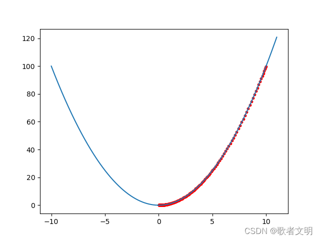
最开始的梯度下降算法，更新权重的方法是theta  = theta - learning_rate * gradient(loss),loss是损失函数。但是这种方法只关心当前的梯度，如果坡度较缓，则它依然会以一种缓慢的速度下降，我们先举个例子，使用梯度下降来寻找y = x*x的最小值。使用z = (x+y)^2当作例子更好点，但是代码也写得多，以后有空再改吧。

代码使用tensorflow实现。

因为用tensorflow的人很少，所以我选择用tensorflow了，开玩笑，开玩笑，是我运气不好，第一次接触深度学习用的是tensorflow，现在用得惯了，tensorflow确实比pytorch麻烦，难矣哉。

def fun(x):
    return x**2
 
 
plt.rcParams['font.family'] = 'DejaVu Sans' 
x = tf.Variable(np.arange(-10.0,11.0,0.01))
plt.plot(x, fun(x))
 
#梯度下降
learning_rate = 0.001#选择学习率
result = []
xlabel = []
y = fun(x)[0]
count = 1
i = tf.Variable(10.0) #初始值
while True and count < 10000:
    with tf.GradientTape() as tape:
        tape.watch(i)
        y = fun(i)
    grad = tape.gradient(y,i)
    if tf.math.less(tf.math.abs(fun(i)), 0.001):
        break
    i = i -  learning_rate * grad
    xlabel.append(i)
    result.append(fun(i))
    count += 1
plt.scatter(xlabel, result, s = 10, c='r')

红色的点是梯度下降过程的寻找过程，它下降了2877次才找到最低点，我们用它来作为对比，这里可以看到，随着越来越接近底部，坡度越来越缓，因此梯度下降越来越慢，我们可以修改学习率使它下降的更快，这里为了对比，选择了较小的学习率

---

2.动量优化

        它是根据之前的梯度来进行计算，每次迭代的时候，它都会从动量向量m种减去局部梯度，然后更新动量向量。

这种方法其实是加速度而不是速度(梯度是速度，加速度就是梯度的梯度)，它要比梯度下降快得多，还能避免局部最小值问题，他的另一个缺点是增加了另一个参数来调整，动量值取0.9一般能够取得很好的效果。

动量优化怎么算?

先求出梯度dw,然后计算动量m，m等于动量常数乘以上一个m减去学习率乘以梯度值

def fun(x):
    return x**2
 
plt.rcParams['font.family'] = 'DejaVu Sans' 
x = tf.Variable(np.arange(-10.0,11.0,0.01))
plt.plot(x, fun(x))
 
 
#动量算法
learning_rate = 0.001
result = []
xlabel = []
y = fun(x)[0]
m = 0#初始化动量为0
beta = 0.9#设置动量大小
i = tf.Variable(10.0) #设置初始位置
count = 1
while True and count < 10000:
    with tf.GradientTape() as tape:
        tape.watch(i)
        y = fun(i)
    grad = tape.gradient(y,i)
    m = beta * m - learning_rate * grad
    i = i + m
    if tf.math.less(tf.math.abs(fun(i)), 0.001):
        print(fun(i))
        break
    count += 1
    xlabel.append(i)
    result.append(fun(i))
plt.scatter(xlabel, result, s = 10, c='r')

最终它只用了230次找到了最小值，中间还有跑过了头，但是最后还是弹跳回到了应该找到的位置

---

3.Nesterov加速梯度

这是动量优化的变体，只多了一个β*m

为什么要使用theta+beta*m呢？

这是因为beta*m的方向是正确的方向，优化的前进方向就是正确的，而且向前迈进了一步，朝着更远的梯度优化，所以速度会更快，

def fun(x):
    return x**2
 
plt.rcParams['font.family'] = 'DejaVu Sans' 
x = tf.Variable(np.arange(-10.0,11.0,0.01))
plt.plot(x, fun(x))
 
 
#动量算法
learning_rate = 0.001
result = []
xlabel = []
y = fun(x)[0]
m = 0#初始化动量为0
beta = 0.9#设置动量大小
i = tf.Variable(10.0) #设置初始位置
count = 1
while True and count < 1000:
    #为了不变更i
    i = i + beta * m#nesterov的不同之处
    with tf.GradientTape() as tape:
        tape.watch(i)
        y = fun(i)
    grad = tape.gradient(y,i)
    m = beta * m - learning_rate * grad
    i = i + m
    if tf.math.less(tf.math.abs(fun(i)), 0.001):
        print(fun(i))
        break
    count += 1
    xlabel.append(i)
    result.append(fun(i))
plt.scatter(xlabel, result, s = 10, c='r')

只用了70次就到达可最小值，据说它还有一个好处，就是在动量过大的时候，弹跳相对于普通动量优化少一些。不过，我觉得这要看情况，不一定绝对好吧。

---

4.Adagrad

梯度下降算法在坡度较为陡的时候，下降很快，到了坡段缓慢的地方下降较慢，说明它没有指向全局的最优解方向。Adagrad算法通过沿最陡的坡度按比例缩小梯度来实现矫正

记住s是一个向量，有多少维度就有多少个向量，公式分解为两步：

(1).s和梯度值的平方对应相加

(2)更新theta的值，看起来与梯度下降完全相同，但是梯度除以s开方了，里面有一个segama数值是防止除数为0的。

这个算法会降低学习率。

这个算法缺陷很多，在一般的深度神经网络中会导致梯度下降提前终止，但是对于一些简单的二次函数，会有不错的效果。

def fun(x):
    return x**2
 
plt.rcParams['font.family'] = 'DejaVu Sans' 
x = tf.Variable(np.arange(-10.0,11.0,0.01))
plt.plot(x, fun(x))
 
#Adagrad
learning_rate = 0.01
result = []
xlabel = []
y = fun(x)[0]
s = 0#初始化动量为0
theta = tf.Variable(0.0)
i = tf.Variable(10.0) #设置初始位置
count = 1
while True and count < 1000:
    with tf.GradientTape() as tape:
        tape.watch(i)
        y = fun(i)
    grad = tape.gradient(y,i)
    s = s + tf.square(grad)
    i = i - learning_rate*grad / tf.sqrt(s + tf.Variable(0.00001))
    if tf.math.less(tf.math.abs(fun(i)), 0.001):
        print(fun(i))
        break
    count += 1
    xlabel.append(i)
    result.append(fun(i))
plt.scatter(xlabel, result, s = 10, c='r')

这里就不给出图了，因为运算很慢。

---

5.RMSProp

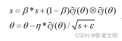
这里的β一般取0.9，这个算法是Adagrad的改善，曾经获得广泛的支持，热度不减

def fun(x):
    return x**2
 
plt.rcParams['font.family'] = 'DejaVu Sans' 
x = tf.Variable(np.arange(-10.0,11.0,0.01))
plt.plot(x, fun(x))
 
#Adagrad
learning_rate = 0.001
result = []
xlabel = []
beta = 0.9
y = fun(x)[0]
s = 0#初始化动量为0
theta = tf.Variable(0.0)
i = tf.Variable(10.0) #设置初始位置
count = 1
while True:
    with tf.GradientTape() as tape:
        tape.watch(i)
        y = fun(i)
    grad = tape.gradient(y,i)
    s = beta * s + (1-beta) * tf.multiply(grad, grad)
    i = i - learning_rate*grad /tf.sqrt(s)
    if tf.math.less(tf.math.abs(fun(i)), 0.001):
        print(fun(i))
        break
    count += 1
    xlabel.append(i)
    result.append(fun(i))
plt.scatter(xlabel, result, s = 10, c='r')

---

6.Adam

这个算法的公式其实只需要修改一下前面的就可以了，其中t代表第t次迭代。

import pandas as pd
import numpy as np
import matplotlib.pyplot as plt
import tensorflow as tf
def fun(x):
    return x**2
 
plt.rcParams['font.family'] = 'DejaVu Sans' 
x = tf.Variable(np.arange(-10.0,11.0,0.01))
plt.plot(x, fun(x))
 
#Adagrad
learning_rate = 0.1
result = []
xlabel = []
beta1 = tf.Variable(0.9)
beta2 = tf.Variable(0.999)
m = 0
s = 0#初始化动量为0
y = fun(x)[0]
count = 1
i = tf.Variable(10.0) #设置初始位置
while True and count < 1000:
    with tf.GradientTape() as tape:
        tape.watch(i)
        y = fun(i)
    grad = tape.gradient(y,i)
    m = beta1 * m + (1-beta1)*grad
    s = beta2 * s + (1-beta2) * grad * grad
    _m = m / (1-tf.pow(beta1,count))
    _s = s/(1-tf.pow(beta2,count))
    i = i - learning_rate * _m /tf.sqrt(_s)
    if tf.math.less(tf.math.abs(fun(i)), 0.001):
        print(fun(i))
        break
    count += 1
    xlabel.append(i)
    result.append(fun(i))
plt.scatter(xlabel, result, s = 10, c='r')

这个算法的麻烦在于需要寻找一个合适的初始化量，比如学习率，这里不继续贴图了，自适应矩阵算法用的更为广泛。beta1和beta2一般被初始化为0.9,和0.999

还有两种值得一看的优化器AdaMax和Nadam,但是在我看来，从RMSprop和Adam族优化器，都比较依赖初始化参数，比如学习率，学习率没有选好，收敛速度可能不如梯度下降，欢迎各位反驳。