深度学习从入门到入土

1. 数据操作和数据预处理

1.1 数据操作

N维数组样例

• N维数组是机器学习和神经网络的主要数据结构

• 0-d

  一个类别： 1.0

• 1-d

  一个特征向量(一维矩阵)：[1.0, 2.7, 3.4]

• 2-d

  一个样本-特征矩阵-(二维矩阵)

• 3-d

  RGB图片 （宽x高x通道）- 三维数组

• 4-d

  一个RGB图片批量（批量大小x宽x高x通道）

• 5-d

  一个视频批量（批量大小x时间x宽x高x通道）

• 创建数组需要：

  • 形状
  • 每个元素的数据类型
  • 每个元素的值

• 访问元素

  • 一个元素 ：[1, 2]
  • 一行：[1, :]
  • 一列：[:, 1]
  • 子区域：[1:3, 1:] (访问到的是1-2行【注意是开区间】，列是访问到底)
  • 子区域：[：：3, ：：2] （访问的是第一行到最后一行，但是每三行一跳，列没两列一跳）

1. 2 数据操作实现

• 首先要导入torch，张量表示要给数值组成的数组，这个数组可能有多个维度

• 可以通过张量的shape属性来访问张量的形状和张量中元素的总数，使用numel来访问张量中的种数

• 要改变一个张量的形状而不改变元素数量和元素值，我们可以调用reshape函数

  

• 使用全0、全1、其他常量或者从特定分布种随机采样的数字- zeros() 和ones()函数

  

• 通过提供包含数值的python列表（或者嵌套列表）来为所需张量中的每个元素赋予确定值

• 常见的标准算数运算符（+，-，*，/，和**【求幂】）都可以被升级为按元素运算

• 按元素方式应用更多的计算

• 也可以将多个张量连接在一起

• 通过逻辑运算符构建二元张量

• 对张量中的所有元素进行求和会产生一个只有一个元素的张量
  
• 即使形状不同，我们任然可以通过调用广播机制（broadcasting mechanism）来执行按元素操作
  只要维度相同，a->(3x2) b->(3x2)
  
• 可以用[-1]选择最后一个元素，可以用[1, 3]选择第二个和第三个元素
  
• 除了读取外，还可以通过指定索引来将元素写入矩阵
  - 为多个元素赋相同的值，只需要索引所有元素，然后为他们赋值
  
• 运行一些操作
  
• 如果后续计算中没有重复使用x，可以使用x[:] = x+Y或者x+=Y来减少操作的内存开销
  
• 转化
  

1. 3 数据预处理实现

• 创建一个人工数据集，并存储在csv（逗号分隔值）文件

import os

os.makedirs(os.path.join('.','data'), exist_ok=True)
data_file = os.path.join('.', 'data', 'house_tiny.csv')
with open(data_file, 'w') as f:
    f.write('NumRooms,Alley,Price\n')
    f.write('NA,Pave,127500\n')
    f.write('2,NA,106000\n')
    f.write('4,NA,178100\n')
    f.write('NA,NA,140000\n')
1
2
3
4
5
6
7
8
9
10

• 从创建的csv文件中加载原始数据集
  
• 安装pandas命令

pip install -i https://pypi.tuna.tsinghua.edu.cn/simple pandas
1

• 成功读取
  
• 为了处理缺失的数据，典型的方法包括 插值和删除
  
• 对于inputs中的类别值或离散值，将NaN视为一个类别
  
• 现在inputs和outputs中的所有条目都是数值类型，它们可以转化为张量格式
  
• 报错，解决方案：使用.astype(“float64”)强制转化
  

2. 线性代数

2.1 线性代数实现

• 标量由只有一个元素的张量表示
  

• 可以将向量视为标量值组成的列表
  

• 通过张量的索引来访问任意元素
  

• 访问张量的长度
  

• 只有一个轴的张量，形状只有一个元素
  

• 通过指定两个分量m和n来创建一个形状为m*n的矩阵

• 矩阵的转置
  

• 对称矩阵symmetric matrix A转置等于其本身
  

• 向量是标量的推广，矩阵是向量的推广，同理可以构建具有更多轴的数据结构
  

• 给定具有相同形状的任何两个张量，任何按元素二元运算的结果都将是相同形状的张量
  

• 两个矩阵的按元素乘法称为哈达玛积（Hadmard product)
  
  
  对X的所有元素都加上a/乘以a

• 计算其元素的和
  

• 表示任意形状张量的元素和
  
  

• 指定求个汇总张量的轴
  axis=0：横向不变，纵向拍扁
  axis=1：纵向不变，横向拍扁
  按照哪个求和就消去哪个轴
  
  

• 一个求和相关的量是平均值（mean或者average）
  

• 计算总和或均值时保持轴数不变(keepdims=True保持轴数不丢)
  

• 某个轴计算A元素的累计总和
  

• 点积是相同位置的按元素乘积的和
  

• 矩阵向量积Ax是一个长度为m的列向量

• 可以将矩阵-矩阵乘法AB看作简单的执行m次矩阵-向量积，并将结果拼在一起，形成一个n*m的矩阵
  
• L2范数是向量元素平方和的平方根
  
• L1范数是向量元素的绝对值之和
  
• 矩阵的 佛罗贝尼乌斯范数（Frobenius norm）是矩阵元素的平方和的平方根
  

3. 矩阵计算

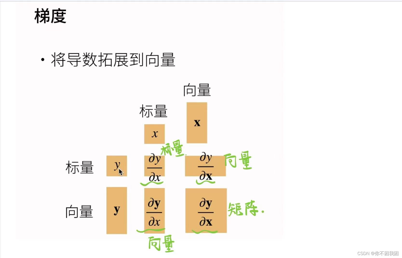
4. 自动求导

• 假设对函数y = 2torch.dot(x, x) 关于列向量x求导
  

• 通过调用反向传播函数来自动计算y关于x的每个分量的梯度
  

• 现在可以计算x的另一个函数
  在默认情况下，pytorch会累计梯度，所以计算新的函数的时候需要清楚之前的值
  

• 深度学习中，主要应用是批量中每个样本单独计算的偏导数之和
  

• 将某些计算移动到记录的计算图之外
  

• 即使构建函数的计算图需要通过Python控制流（例如：条件、循环或者任意函数调用）,任然可以计算得到的变量的梯度
  
  即使流程控制产生了不同的函数公式，但是每次计算的时候，pytorch都会把计算图给存起来

5. 线性回归+基础优化算法

5.1 线性回归

• 线性回归是对n维输入的加权，外加偏差
• 使用平方损失来衡量预测值和真实值的差异
• 线性回归有显式解
• 线性回归可以看作是单层神经网络

5.2 基础优化算法

• 梯度下降通过不断沿着反梯度方向更新参数求解
• 小批量随机梯度下降是深度学习默认的求解算法
• 两个重要的超参数是批量大小和学习率
  

5.3 线性回归的从0开始实现

• 数据流水线、模型、损失函数和小批量随机梯度下降优化器
• 下载matplotlib

pip install -i https://pypi.tuna.tsinghua.edu.cn/simple matplotlib==3.5.0
1

• d2l报错，重下

pip install -i https://pypi.tuna.tsinghua.edu.cn/simple d2l torch torchvision
1

实现完整示例：

#import matplotlib.pyplot as plt
%matplotlib inline
import random
import torch
from d2l import torch as d2l

# 自定义随机样本
def synthetic_data(w, b, num_examples):
    """生成 y = Xw + b + 噪声"""
    """
    X:均值为0，方差为1的随机数
    """
    X = torch.normal(0, 1, (num_examples, len(w)))
    y = torch.matmul(X, w) + b
    """加入随机噪音"""
    y += torch.normal(0, 0.01, y.shape)
    """返回列向量"""
    return X, y.reshape((-1, 1))

true_w = torch.tensor([2, -3.4])
true_b = 4.2
features, labels = synthetic_data(true_w, true_b, 1000)

# 定义一个data_iter函数，该函数接受批量大小、特征矩阵和标量向量作为输入，生成大小为batch_size的小批量
def data_iter(batch_size, features, labels):
    num_examples = len(features)
    indices = list(range(num_examples))
    # 这些样本是随机读取的，没有特定的顺序
    random.shuffle(indices)
    for i in range(0, num_examples, batch_size):
        batch_indices = torch.tensor(indices[i:min(i + batch_size, num_examples)])# 每次拿一定批量的数据
        yield features[batch_indices], labels[batch_indices]

batch_size = 10
for X, y in data_iter(batch_size, features, labels):
    print(X, '\n', y)
    break
    
# 定义初始化模型参数
w = torch.normal(0, 0.01, size=(2, 1), requires_grad= True)# 输入维度为长为2的向量，随机初始化为均值为0，方差为0.01的正态分布
b = torch.zeros(1, requires_grad=True)# 偏差定义为0的标量

# 定义模型
def linreg(X, w, b):
    """线性回归模型"""
    return torch.matmul(X, w) + b
   
# 定义损失函数
def squared_loss(y_hat, y):# y_hat预测值，y真实值
    """均方损失"""
    return (y_hat - y.reshape(y_hat.shape))**2 / 2
# 定义优化算法
def sgd(params, lr, batch_size): # params：所有参数的集合，包括w和b， lr:学习率
    """小批量随机梯度下降"""
    with torch.no_grad():
        for param in params:
            param -= lr * param.grad / batch_size# 求均值
            param.grad.zero_()# 确保下次梯度计算不会受影响
# 训练过程
"""定义相应超参数"""
lr = 0.001
num_epochs = 10
net = linreg
loss = squared_loss

for epoch in range(num_epochs):
    for X, y in data_iter(batch_size, features, labels):
        """
        X 和 y的小批量损失，因为 l 的形状是(batch_size, 1)而不是一个标量
        并以此计算关于[w, b]的梯度
        """
        l = loss(net(X, w, b), y)
        l.sum().backward() # 求和之后算梯度
        sgd([w, b], lr, batch_size) # 使用[w, b]更新参数
        
    with torch.no_grad():
        train_l = loss(net(features, w, b), labels)
        print(f'epoch{epoch + 1}, loss{float(train_l.mean()):f}')

# 比较真实参数和通过训练学到的参数来评估训练的成功程度
print(f'w的估计误差：{true_w - w.reshape(true_w.shape)}')
print(f'b的估计误差：{true_b - b}')
1
2
3
4
5
6
7
8
9
10
11
12
13
14
15
16
17
18
19
20
21
22
23
24
25
26
27
28
29
30
31
32
33
34
35
36
37
38
39
40
41
42
43
44
45
46
47
48
49
50
51
52
53
54
55
56
57
58
59
60
61
62
63
64
65
66
67
68
69
70
71
72
73
74
75
76
77
78
79
80
81
82

实现：

features 中的每一行都包含一个二维数据样本，labels中的每一行都包含一维标签值（一个标量），可以通过d2l查看训练样本

• 定义一个data_iter函数，该函数接受批量大小、特征矩阵和标量向量作为输入，生成大小为batch_size的小批量
  

• 定义初始化模型参数
  

• 定义模型
  

• 定义损失函数
  

• 定义优化算法
  

• 训练过程
  

• 比较真实参数和通过训练学到的参数来评估训练的成功程度
  

• 对于一些超参数的调整

  • lr过小，损失太大，需要跑很多轮才能降下来
    

5.4 线性回归的简捷实现

import numpy as np
import torch
from torch.utils import data
from d2l import torch as d2l 
from torch import nn

true_w = torch.tensor([2, -3.4])
true_b = 4.2
features, labels = d2l.synthetic_data(true_w, true_b, 1000)

# 调用框架中现有的API来读取数据
def load_array(data_arrays, batch_size, is_train=True):
    """构造一个PyTorch数据迭代器"""
    dataset = data.TensorDataset(*data_arrays)
    return data.DataLoader(dataset, batch_size, shuffle=is_train)
batch_size = 10
data_iter = load_array((features, labels), batch_size)

next(iter(data_iter))

# 使用框架的预定义好的层
net = nn.Sequential(nn.Linear(2, 1))# .Linear(输入维度, 输出维度)

# 初始化模型参数
net[0].weight.data.normal_(0, 0.01)
net[0].bias.data.fill_(0)

# 计算均方误差使用的是MSELoss类，也称为平方范数
loss = nn.MSELoss()

# 实例化SGD实例
trainer = torch.optim.SGD(net.parameters(), lr=0.03)

# 训练过程
num_epochs = 5
for epoch in range(num_epochs):
    for X, y in data_iter:
        l = loss(net(X), y) # net本身带有模型参数
        trainer.zero_grad()
        l.backward()
        trainer.step() # .step()进行模型的更新
    l = loss(net(features), labels)
    print(f'epoch{epoch + 1}, loss{l:f}')
1
2
3
4
5
6
7
8
9
10
11
12
13
14
15
16
17
18
19
20
21
22
23
24
25
26
27
28
29
30
31
32
33
34
35
36
37
38
39
40
41
42
43

• 可以通过使用深度学习框架来简洁地实现 线性回归模型 生成数据集
  
• 调用框架中现有的API来读取数据
  
• 使用框架的预定义好的层
  
• 初始化模型参数
  
• 计算均方误差使用的是MSELoss类，也称为平方范数
• 实例化SGD实例
  
• 训练过程
  

6. Softmax回归

6.1 Softmax回归

• 分类和回归的区别
  • 回归：估计一个连续值
  • 分类：预测一个离散类别
• 从回归到多类别分类

• 从回归到多类分类->均方损失

  • 对类别进行一位有效编码
  • 使用均方损失训练
  • 最大值作为预测
    

• 从回归到多类分类->无校验比例（合适的区间）

  • 对类别进行一位有效编码
  • 最大值作为预测
  • 需要更置信的识别正确类（大余量）

• 从回归到多类分类->校验比例

  • 输出匹配概率（非负，和为1）

- 概率y和y‘的区别作为损失

- Softmax和交叉熵损失
1

• 总结：

  • Softmax回归是一个多类分类模型
  • 使用Softmax操作子得到每个类的预测置信度
  • 使用交叉熵来衡量预测和标号的区别

6.2 损失函数

6.3 图片分类数据集

• MNIST数据集是图像分类中广泛使用的数据集之一，但作为基准数据集过于简单，所有使用类似但更复杂的Fasion-MNIST数据集
  

• 通过框架中的内置函数将Fasion-MNIST数据集下载并读取到内存中
  测试数据集不参与训练，主要用来测试模型的好坏
  
  
  查看第一张图片，因为是黑白，所以通道数为1

• 两个可视化数据集的函数
  

• 几个样本的图像以及其相应的标签
  
  

• 读取一小批量数据，大小为batch_size
  

• 定义load_data_fasion_mnist函数进行功能的封装
  

6.4 softmax回归的从0开始实现

• 将展平每个图像，将它们视为长度为784（28*28）的向量，因为数据集有10个类别，所以网络输出维度为10

  • 行数为784， 列数为10， 因为要计算梯度所以require——grad设置为True
  • b为偏移

  

• 给定一个矩阵x，可以对所有元素求和(具体可见前面章节)
  

• 实现softmax
  

• 进行简单的验证：将每个元素变成一个非负数，此外，根据概率原理，每行总和为1
  
• 实现softmax回归模型
  
• 创建一个数据y_hat， 其中包含2个样本在3个类别的预测概率，使用y作为y_hat中概率的索引
  
• 实现交叉熵损失函数
  
  得到样本0和样本1的损失
  
• 因为做的是分类问题，所以要用预测值和真实值y元素进行比较
  
• 可以评估在任意模型net的准确率

def evaluate_accuarcy(net, data_iter):
    """计算在指定的数据集上模型的精度"""
    if isinstance(net, torch.nn.Module):
        net.eval()# 将模型设置为评估模式（不计算梯度）
    metric = Accumulator(2)# 正确预测数、预测总数放入metric迭代器
    for X, y in data_iter:
        metric.add(accuracy(net(X), y), y.numel())
    return metric[0] / metric[1]# 分类正确的样本数 / 总样本数
1
2
3
4
5
6
7
8

• Accumulator实例中创建了两个变量，用于分别存储正确预测的数量和预测的总数量

class Accumulator:
    """在n个变量上累加"""
    def __init__(self, n):
        self.data = [0.0] * n
    
    def add(self, *args):
        self.data = [a + float(b) for a, b in zip(self.data, args)]
    
    def reset(self):
        self.data = [0.0] * len(self.data)
    
    def __getitem__(self, idx):
        return self.data[idx]

evaluate_accuarcy(net, test_iter)
1
2
3
4
5
6
7
8
9
10
11
12
13
14
15

因为是十分类，任意网络下结果是随机的正确率接近1/10

• Softmax回归的训练

def train_epoch_ch3(net, train_iter, loss, updater):  
    """训练模型一个迭代周期"""
    if isinstance(net, torch.nn.Module):
        net.train()
    metric = Accumulator(3)
    for X, y in train_iter:
        y_hat = net(X)
        l = loss(y_hat, y)
        if isinstance(updater, torch.optim.Optimizer):
            # 使用PyTorch内置的优化器和损失函数
            updater.zero_grad()
            l.backward() # 计算梯度
            updater.step()# 对参数进行更新
            metric.add(
                float(l) * len(y), accuracy(y_hat, y), y.size().numel())#把正确的样本数放入累加器
        else:
            # 使用自定义的损失函数
            l.sum().backward() # 先求和再计算梯度
            updater(X.shape[0])
            metric.add(float(l.sum()), accuracy(y_hat, y), y.numel())
    return metric[0] / metric[2], metric[1] / metric[2]# 损失的累加/样本数-》训练损失，分类正确/总样本数-》训练精度

# 定义一个再动画中绘制数据的实用程序类
class Animator:  #用一个小动画让你看到在训练过程中的变化，不解释了，用matplotlip画图
    """在动画中绘制数据"""
    def __init__(self, xlabel=None, ylabel=None, legend=None, xlim=None,
                 ylim=None, xscale='linear', yscale='linear',
                 fmts=('-', 'm--', 'g-.', 'r:'), nrows=1, ncols=1,
                 figsize=(3.5, 2.5)):
        # 增量地绘制多条线
        if legend is None:
            legend = []
        d2l.use_svg_display()
        self.fig, self.axes = d2l.plt.subplots(nrows, ncols, figsize=figsize)
        if nrows * ncols == 1:
            self.axes = [self.axes, ]
        # 使用lambda函数捕获参数
        self.config_axes = lambda: d2l.set_axes(
            self.axes[0], xlabel, ylabel, xlim, ylim, xscale, yscale, legend)
        self.X, self.Y, self.fmts = None, None, fmts
 
    def add(self, x, y):
        # 向图表中添加多个数据点
        if not hasattr(y, "__len__"):
            y = [y]
        n = len(y)
        if not hasattr(x, "__len__"):
            x = [x] * n
        if not self.X:
            self.X = [[] for _ in range(n)]
        if not self.Y:
            self.Y = [[] for _ in range(n)]
        for i, (a, b) in enumerate(zip(x, y)):
            if a is not None and b is not None:
                self.X[i].append(a)
                self.Y[i].append(b)
        self.axes[0].cla()
        for x, y, fmt in zip(self.X, self.Y, self.fmts):
            self.axes[0].plot(x, y, fmt)
        self.config_axes()
        display.display(self.fig)
        display.clear_output(wait=True)
1
2
3
4
5
6
7
8
9
10
11
12
13
14
15
16
17
18
19
20
21
22
23
24
25
26
27
28
29
30
31
32
33
34
35
36
37
38
39
40
41
42
43
44
45
46
47
48
49
50
51
52
53
54
55
56
57
58
59
60
61
62

• 训练函数

def train_ch3(net, train_iter, test_iter, loss, num_epochs, updater):  
    """训练模型"""
    animator = Animator(xlabel='epoch', xlim=[1, num_epochs], ylim=[0.3, 0.9],
                        legend=['train loss', 'train acc', 'test acc'])# 可视化
    for epoch in range(num_epochs):
        train_metrics = train_epoch_ch3(net, train_iter, loss, updater)
        test_acc = evaluate_accuracy(net, test_iter)# 在测试数据集上更新精度
        animator.add(epoch + 1, train_metrics + (test_acc,))
    train_loss, train_acc = train_metrics
    assert train_loss < 0.5, train_loss
    assert train_acc <= 1 and train_acc > 0.7, train_acc
    assert test_acc <= 1 and test_acc > 0.7, test_acc
1
2
3
4
5
6
7
8
9
10
11
12

• 小批量随机梯度下降来优化模型的损失函数

lr = 0.1

def updater(batch_size):
    return d2l.sgd([W, b], lr, batch_size)
1
2
3
4

• 训练模型10个迭代周期

num_epochs = 10 #训练10个迭代周期
train_ch3(net, train_iter, test_iter, cross_entropy, num_epochs, updater)
1
2

结果：

• 对图像进行分类预测

def predict_ch3(net, test_iter, n=6):  
    """预测标签"""
    for X, y in test_iter: # 从测试数据集中拿出一个样本
        break
    trues = d2l.get_fashion_mnist_labels(y)# 拿出真实标签值
    preds = d2l.get_fashion_mnist_labels(net(X).argmax(axis=1)) # 拿出预测标签值
    titles = [true + '\n' + pred for true, pred in zip(trues, preds)]
    d2l.show_images(X[0:n].reshape((n, 28, 28)), 1, n, titles=titles[0:n])

predict_ch3(net, test_iter)
1
2
3
4
5
6
7
8
9
10

预测结果：

6.5 Softmax回归的简洁实现

使用深度学习框架的高级API使得实现softmax更加容易

import torch
from torch import nn
from d2l import torch as d2l

batch_size = 256
train_iter, test_iter = load_data_fashion_mnist(batch_size) # 把训练数据和测试数据放到迭代器中
1
2
3
4
5
6

Softmax回归的输出层是一个全连接层，完成初始化

# PyTorch不会隐式地调整输入的形状
# 因此，定义了展平层（flatten）在线性层前调整网络输入的形状
net = nn.Sequential(nn.Flatten(), nn.Linear(784, 10))

def init_weights(m):
    if type(m) == nn.Linear:
        nn.init.normal_(m.weight, std=0.01)
    
net.apply(init_weights)
1
2
3
4
5
6
7
8
9

在交叉熵损失函数中传递未归一化的预测，并同时计算softmax及其对数

loss = nn.CrossEntropyLoss()
1

使用学习率未0.1的小批量随机梯度下降作为优化算法

trainer = torch.optim.SGD(net.parameters(), lr=0.1)
1

调用之前定义的训练函数来训练模型

num_epochs = 10
train_ch3(net, train_iter, test_iter, loss, num_epochs, trainer)
1
2

7. 感知机

7.1 感知机

• 感知机是一个二分类模型，是最早的AI模型之一
• 它的求解算法等价于使用批量为1的梯度下降
• 不能拟合XOR函数

7.2 多层感知机

• 多层感知机使用隐藏层和激活函数来得到非线性模型
• 常用的激活函数是Sigmoid Tanh ReLU
• 使用Softmax来处理多类分类
• 超参数为隐藏层数，和各个隐藏层大小

7.3 多层感知机的从0开始实现

import torch
from torch import nn
from d2l import torch as d2l

batch_size = 256
train_iter, test_iter = d2l.load_data_fashion_mnist(batch_size)
1
2
3
4
5
6

• 实现一个具有单隐藏层的多层感知机，它包含256个隐藏单元

num_inputs, num_outputs, num_hiddens = 784, 10, 256 # 输入28*28，输出10分类，隐藏层数作为超参数可以自定义 

W1 = nn.Parameter(
    torch.randn(num_inputs, num_hiddens, requires_grad=True) * 0.01) # 行数784，列数10，梯度
b1 = nn.Parameter(torch.zeros(num_hiddens, requires_grad=True))

W2 = nn.Parameter(
    torch.randn(num_hiddens, num_outputs, requires_grad=True) * 0.01)# 前一个隐藏层的作为输入
b2 = nn.Parameter(torch.zeros(num_outputs, requires_grad=True))

params = [W1, b1, W2, b2]
1
2
3
4
5
6
7
8
9
10
11

• 实现ReLU激活函数

def relu(X):
    a = torch.zeros_like(X)
    return torch.max(X, a)
1
2
3

• 实现模型

def net(X):
    X = X.reshape((-1, num_inputs))
    H = relu(X @ W1 + b1) # 矩阵乘法
    return (H @ W2 + b2)

loss = nn.CrossEntropyLoss()
1
2
3
4
5
6

• 多层感知机的训练过程与softmax回归的训练过程完全相同

loss = nn.CrossEntropyLoss()
num_epochs, lr = 25, 0.1
updater = torch.optim.SGD(params, lr=lr)
d2l.train_ch3(net, train_iter, test_iter, loss, num_epochs, updater)
1
2
3
4

8. 模型选择和过拟合

8.1 模型选择

• 训练误差：模型在训练数据上的误差

• 泛化误差：模型在新数据上的误差（真正应该关注的误差）

• 验证数据集：一个用来评估模型好坏的数据集（不参与训练）

  • 注意：不要和训练数据混在一起使用

    不能用于调参，只能评估模型好坏

• 测试数据集：只能使用一次的数据集

• 训练数据集：训练模型参数

• K-则交叉验证

  • 在没有足够多的数据时使用

  • 算法：

    for i = 1，…K

    将训练数据分割成K块，使用第i块作为验证数据集，其余作为训练数据集

    报告K个验证集误差的平均

8.2 过拟合和欠拟合

• 模型容量：拟合各种函数的能力

低容量的模型难以拟合训练数据

高容量的模型可以记住所有训练数据

• 模型容量的影响：
  

• 估计模型容量

  • 难以在不同种类算法之间比较
  • 给定一个模型种类，将有两个主要因素：参数的个数、参数值的选择范围

• VC维：在深度学习中很少使用，因为参数计算困难

• 模型容量需要匹配数据复杂度，否则可能会导致欠拟合或者过拟合

• 统计机器学习提供数学工具来衡量模型复杂度

• 实际中一般靠观察训练误差和验证误差

8.3 实现

1 模型选择、欠拟合和过拟合

通过多项式拟合来交互地探索这些概念

import math
import numpy as np
import torch
from torch import nn
from d2l import torch as d2l
1
2
3
4
5

使用以下三阶多项式来生成训练和测试数的标签
$$y=5+1.2x-3.4\frac{x^2}{2!}+5.6\frac{x^3}{3!}+ϵwhereϵ\sim N(0,0.1^2)$$

【np.random.normal函数用来生成服从均值为0、标准差为1的标准正态分布的随机数。它的第一个参数是size，用来指定生成随机数的个数和维度】

max_degree = 20 # 最高次数的多项式特征为20
n_train, n_test = 100, 100 # 用100个训练样本，100个测试样本（用以验证）
true_w = np.zeros(max_degree) # 展开的真实值为20维
true_w[0:4]=np.array([5, 1.2, -3.4, 5.6])# 前四位自定，后面所有均为0（作为噪音项）

features = np.random.normal(size=(n_train + n_test, 1)) # 生成服从正态分布的随机数，features是一个形状为(n_train + n_test, 1)的数组，它将包含n_train + n_test个服从标准正态分布的随机数
np.random.shuffle(features) # 打乱数组features的顺序
poly_features = np.power(features, np.arange(max_degree).reshape(1, -1))# 存放所有样本的x的阶乘结果，格式为200*20
"""
对poly_features中的每一列进行归一化处理，使得每个特征都除以相应的阶乘值
具体来说，代码中的循环遍历了max_degree这个范围，对于每一个阶数i，将poly_features中的第i列除以math.gamma(i + 1)。
math.gamma函数，它计算i + 1的阶乘值。
通过除以相应的阶乘值，可以确保每个特征都被正确归一化，避免了因为高阶项的数值较大导致特征的不平衡问题
"""
for i in range(max_degree):
    poly_features[:, i] /= math.gamma(i + 1)

"""
通过np.dot()函数进行矩阵乘法操作，将多项式特征矩阵的每一行与真实权重向量进行乘法运算，得到对应的标签值
"""
labels = np.dot(poly_features, true_w)
"""
每个标签添加了服从均值为0、标准差为0.1的正态分布噪声。
具体来说，通过np.random.normal(scale=0.1, size=labels.shape)生成了一个具有与labels相同形状的随机数数组作为噪声，
然后将该噪声加到原始的labels数组上。"""
labels += np.random.normal(scale=0.1, size=labels.shape)
1
2
3
4
5
6
7
8
9
10
11
12
13
14
15
16
17
18
19
20
21
22
23
24
25
26

看一下前2个样本

# 将原始数据类型转化为tensor
true_w, features, poly_features, labels = [
    torch.tensor(x, dtype=torch.float32)
    for x in [true_w, features, poly_features, labels]]

features[:2], poly_features[:2, :], labels[:2]
1
2
3
4
5
6

实现一个函数来评估模型在给定数据集上的损失

def evaluate_loss(net, data_iter, loss):
"""
Accumulator(2)创建了一个metric累加器对象，并指定了累加器的大小为2。
这意味着metric累加器将用于累积两个值。
"""
    metric = d2l.Accumulator(2)
    for X, y in data_iter:
        out = net(X)
        y = y.reshape(out.shape)
        l = loss(out, y)
        metric.add(l.sum(), l.numel())
    return metric[0]/metric[1]
1
2
3
4
5
6
7
8
9
10
11
12

定义训练数据
【nn.Sequential是PyTorch中的一个模型容器，用于按照顺序组织神经网络的各个层。每个层可以是全连接层、卷积层、激活函数等。】
【nn.Linear是PyTorch中的一个线性层（全连接层）模块。它接收一个参数in_features，表示输入的特征数，和一个参数out_features，表示输出的特征数。此外，bias参数表示是否包含偏置项。】

def train(train_features, test_features, train_labels, test_labels,num_epochs=400):
    loss = nn.MSELoss()
    input_shape = train_features.shape[-1]
    # 创建了一个只有一层的神经网络
    net = nn.Sequential(nn.Linear(input_shape, 1, bias=False))# 定义了一个线性层，输入特征数为input_shape，输出特征数为1，并且没有偏置项。
    batch_size = min(10, train_labels.shape[0])
    
    # 数据加载进容器
    train_iter = d2l.load_array((train_features, train_labels.reshape(-1, 1)),
                                batch_size, is_train=True)
    test_iter = d2l.load_array((test_features, test_labels.reshape(-1, 1)),
                               batch_size, is_train=False)
    trainer = torch.optim.SGD(net.parameters(), lr=0.01)# 使用SGD优化
    animator = d2l.Animator(xlabel='epoch', ylabel='loss', yscale='log',
                            xlim=[1, num_epochs], ylim=[1e-3, 1e2],
                            legend=['train', 'test'])
    for epoch in range(num_epochs):
        d2l.train_epoch_ch3(net, train_iter, loss, trainer)
        if epoch == 0 or (epoch + 1) % 20 == 0:
            animator.add(epoch + 1, (evaluate_loss(
                net, train_iter, loss), evaluate_loss(net, test_iter, loss)))
    print('weight:', net[0].weight.data.numpy())
1
2
3
4
5
6
7
8
9
10
11
12
13
14
15
16
17
18
19
20
21
22

• 三项多项式函数拟合（正态）：只使用前4维数据训练

train(poly_features[:n_train, :4], poly_features[n_train:, :4],
      labels[:n_train], labels[n_train:])
1
2

400轮后损失较小

• 线性函数拟合（欠拟合）只用前2个数据进行训练

train(poly_features[:n_train, :2], poly_features[n_train:, :2],
      labels[:n_train], labels[n_train:])
1
2

由于数据没有给全，导致最后gap依然很大

• 高阶多项式函数拟合（过拟合）：把整个20维数据全部投入训练

train(poly_features[:n_train, :], poly_features[n_train:, :],
      labels[:n_train], labels[n_train:], num_epochs=1500)
1
2

过于关注细节导致泛化误差不降反升

9. 权重衰退

9.1 权重衰退基本概念

权重衰减（Weight Decay）是一种用来减小模型复杂度和缓解过拟合问题的正则化方法。它在损失函数中添加了一个正则化项，用于惩罚模型的权重（参数）的大小。

在训练模型时，通常会使用损失函数来度量模型预测与实际观测值之间的差距。权重衰减通过在损失函数中增加一个权重的平方和来惩罚较大的权重值，使模型倾向于选择更小的权重值，从而降低模型复杂度。

权重衰减的基本思想是优化算法在更新模型参数时，不仅要考虑减小损失函数的值，还要尽量减小权重的大小。这有助于减少模型对训练数据的过拟合，并提高模型在未见过的数据上的泛化能力。
解决过拟合的方法：

使用均方范数作为硬性限制

• 通过限制参数值的选择范围来控制模型容量

$$minl(w,b)subjectto||w|{|}^2\le \theta$$

• 通常不限制偏移b
• 小的$\theta$意味着更强的正则项（限制更强）

使用均方范数作为柔性限制

• 对于每个$\theta$，都可以找到$\lambda$使得之前的目标函数等价于下面：
  $$\min l(w,b)+\frac{\lambda }{2}|w|{|}^2$$
• 超参数$\lambda$控制正则项的重要程度
  • $\lambda$=0 无作用
  • $\lambda$->无穷， 限制最强

总结：

• 权重衰退通过L2正则项使得模型参数不会过大，从而控制模型复杂度
• 正则项权重是控制模型复杂度的超参数

9.2 权重衰退的从0实现

%matplotlib inline
import torch 
from torch import nn
from d2l import torch as d2l
1
2
3
4

生成一些数据
$$y=0.05+\sum _{i=1}^{d}0.01x_i+ϵwhereϵ\sim N(0,0.01^2)$$

n_train, n_test, num_inputs, batch_size = 20, 100, 200, 5# 训练样本控制很小，数据越简单，模型越复杂，容易发生过拟合
true_w, true_b = torch.ones((num_inputs, 1)) * 0.01, 0.05
train_data = d2l.synthetic_data(true_w, true_b, n_train)# 创建一个合成的训练数据集
train_iter = d2l.load_array(train_data, batch_size) # 读取
test_data = d2l.synthetic_data(true_w, true_b, n_test)
test_iter = d2l.load_array(test_data, batch_size, is_train=False)
1
2
3
4
5
6

初始化模型参数

def init_params():
    w = torch.normal(0, 1, size=(num_inputs, 1), requires_grad=True)
    b = torch.zeros(1, requires_grad=True) # b作为偏移是全0的标量
    return [w, b]
1
2
3
4

定义L2范数惩罚

def l2_penalty(w):
    return torch.sum(w.pow(2)) / 2
1
2

定义训练代码实现

def train(lambd):
    w, b = init_params()# 初始化权重和偏移
    """
    接受一个参数X，并调用了d2l.linreg(X, w, b)函数。
    lambda函数的返回值就是d2l.linreg(X, w, b)函数的返回值。
    使用平方损失函数
    """
    net, loss = lambda X: d2l.linreg(X, w, b), d2l.squared_loss
    num_epochs, lr = 100, 0.003 # 迭代100次，学习率设置为0.003
    
    animator = d2l.Animator(xlabel='epochs', ylabel='loss', yscale='log',
                            xlim=[5, num_epochs], legend=['train', 'test'])# 可视化一下结果
    for epoch in range(num_epochs):# 每次数据迭代
        for X, y in train_iter: # 每次从迭代器中取出X 和y
            # with torch.enable_grad():
            """
            相比于传统算损失只有loss(net(X), y),权重衰退加上了lambd（标量）* l2_penalty(w)
            """
            l = loss(net(X), y) + lambd * l2_penalty(w)# 损失
            l.sum().backward()# 求梯度
            d2l.sgd([w, b], lr, batch_size)# 优化
        if (epoch + 1) % 5 == 0:
            animator.add(epoch + 1, (d2l.evaluate_loss(net, train_iter, loss),
                                     d2l.evaluate_loss(net, test_iter, loss)))
    print('w的L2范数是：', torch.norm(w).item())
1
2
3
4
5
6
7
8
9
10
11
12
13
14
15
16
17
18
19
20
21
22
23
24
25

忽略正则化直接训练（完全没有L2范数限制）

train(lambd=0)
1

明显过拟合（一直在训练，但是在验证集上基本没有任何进展）
使用权重衰退

train(lambd=3)
1

继续调Lambd

train(lambd=100)
1

欠拟合，还可以通过调整训练样本数和训练轮数来改善拟合状态

9.3 简洁实现

【torch.optim.SGD函数用于创建一个SGD优化器对象，该对象会在训练过程中更新模型的参数】
torch.optim.SGD函数的参数如下：

• params：一个包含要优化的模型参数的列表（或字典）。在这个例子中，列表中包含两个元素，分别代表网络net的第一个层的权重（net[0].weight）和偏置（net[0].bias）参数。
• lr：学习率（learning rate），代表每次参数更新的步长或者学习的速率。
• weight_decay：权重衰减（weight decay）参数，用于控制模型参数的正则化-》lambd

def train_concise(wd):
    net = nn.Sequential(nn.Linear(num_inputs, 1))# 定义线性网络
    for param in net.parameters():
        param.data.normal_()
    loss = nn.MSELoss()# 损失
    num_epochs, lr = 100, 0.003
    # 优化
    trainer = torch.optim.SGD(
        [{ "params": net[0].weight,'weight_decay': wd}, # 权重衰减（weight decay）参数【lamdb】，用于控制模型参数的正则化
        { "params": net[0].bias}], 
        lr=lr)
    # 可视化
    animator = d2l.Animator(xlabel='epochs', ylabel='loss', yscale='log',
                            xlim=[5, num_epochs], legend=['train', 'test'])
    
    for epoch in range(num_epochs):
        for X, y in train_iter:
            with torch.enable_grad():
                trainer.zero_grad() # 重置梯度
                l = loss(net(X), y) # 求损失
            l.backward() # 求梯度
            trainer.step()
        if (epoch + 1) % 5 == 0:
            animator.add(epoch + 1, (d2l.evaluate_loss(net, train_iter, loss),
                                     d2l.evaluate_loss(net, test_iter, loss)))
    print('w的L2范数：', net[0].weight.norm().item())
1
2
3
4
5
6
7
8
9
10
11
12
13
14
15
16
17
18
19
20
21
22
23
24
25
26

train_concise(0)
1

train_concise(3)
1

10. 丢弃法

10.1 基础概念

动机：一个好的模型需要对输入数据的扰动鲁棒

• 使用有噪音的数据等价于Tikhonov正则
• 丢弃法：在层（一般是在MLP的隐藏层输出上）之间加入噪音

无差别的加入噪音

• 对x加入噪音得到$x^{\prime }$，希望
  $$E\left[x^{\prime }\right]=x$$
• 丢弃法对每个元素做如下扰动
  x i ′ = { 0 p x i 1 − p x _ { i } ^ { \prime } = \{ 0pxi1−p xi′​={01−pxi​​​p​
  【注意】除以1-p是为了保证整体期望不变
  使用丢弃法
  通常将丢弃法作用在隐藏全连接层的输出上
  推理中的丢弃法
• 正则项只在训练中使用：它们影响模型参数的更新
• 在推理（预测）过程中，丢弃法直接返回输入

总结：

• 丢弃法将一些输出项随机置0来控制模型复杂度
• 常作用在MLP的隐藏层输出上
• 丢弃概率（p）是控制模型复杂度的超参数

10.2 Dropout的从0开始实现

实现dropout_layer函数，该函数以dropout的概率丢弃张量输入X中的元素
【torch.randn函数生成一个服从标准正态分布（均值为0，标准差为1）的随机张量】

import torch
from torch import nn
from d2l import torch as d2l

def dropout_layer(X, dropout):
    assert 0 <= dropout <= 1
    if dropout == 1:
        return torch.zeros_like(X) # 返回和X shape相同的0
    if dropout == 0:
        return X # 不丢，返回X本身
    """
    torch.randn(X.shape)：此部分创建了一个与输入张量X具有相同形状的随机张量。
    (torch.randn(X.shape) > dropout)将随机张量与一个阈值dropout进行比较，创建了一个布尔型张量，其中大于dropout的元素设为True，小于或等于dropout的元素设为False
    .float()：将布尔型张量转换为浮点型张量
    """
    mask = (torch.randn(X.shape) > dropout).float() # 根据某个阈值（dropout）生成一个与输入张量相同形状的浮点型张量
    # 做乘法比选择元素快，所以不用X[mask]=0
    return mask * X / (1.0 - dropout)
1
2
3
4
5
6
7
8
9
10
11
12
13
14
15
16
17
18

测试dropout_layer函数

X = torch.arange(16, dtype=torch.float32).reshape((2, 8))
print(X)
print(dropout_layer(X, 0.))
print(dropout_layer(X, 0.5))
print(dropout_layer(X, 1.))
1
2
3
4
5

定义具有两个隐藏层的MLP，每个隐藏层包含256个单元

num_inputs, num_outputs, num_hiddens1, num_hiddens2 = 784, 10, 256, 256

dropout1, dropout2 = 0.2, 0.5

class Net(nn.Module):
    def __init__(self, num_inputs, num_outputs, num_hiddens1, num_hiddens2,
                 is_training=True): 
        super(Net, self).__init__() # 复用父函数初始化
        self.num_inputs = num_inputs 
        self.training = is_training # 训练
        self.lin1 = nn.Linear(num_inputs, num_hiddens1)
        self.lin2 = nn.Linear(num_hiddens1, num_hiddens2)
        self.lin3 = nn.Linear(num_hiddens2, num_outputs)
        self.relu = nn.ReLU() # 创建了一个ReLU激活函数对象

    def forward(self, X):
        H1 = self.relu(self.lin1(X.reshape((-1, self.num_inputs))))
        if self.training == True: # 确保是在训练状态下，否则不作用直接输出输出H1
            H1 = dropout_layer(H1, dropout1) # 进行随机概率丢弃
        H2 = self.relu(self.lin2(H1))
        if self.training == True:
            H2 = dropout_layer(H2, dropout2)
        out = self.lin3(H2)
        return out

net = Net(num_inputs, num_outputs, num_hiddens1, num_hiddens2)
1
2
3
4
5
6
7
8
9
10
11
12
13
14
15
16
17
18
19
20
21
22
23
24
25
26

训练和测试

num_epochs, lr, batch_size = 10, 0.5, 256
loss = nn.CrossEntropyLoss()
train_iter, test_iter = d2l.load_data_fashion_mnist(batch_size)
trainer = torch.optim.SGD(net.parameters(), lr=lr)
train_ch3(net, train_iter, test_iter, loss, num_epochs, trainer)
1
2
3
4
5

10.3 简洁实现

【net.apply()函数允许您对神经网络模型的所有子模块进行递归地操作。通过指定一个初始化函数作为参数，模型会遍历自身的所有子模块，并对每个子模块的参数应用初始化函数】

net = nn.Sequential(nn.Flatten(), nn.Linear(784, 256), nn.ReLU(),
                    nn.Dropout(dropout1), nn.Linear(256, 256), nn.ReLU(), # 添加了.Dropout()
                    nn.Dropout(dropout2), nn.Linear(256, 10))

def init_weights(m):
    if type(m) == nn.Linear:
        nn.init.normal_(m.weight, std=0.01)

net.apply(init_weights) # 会遍历神经网络的所有模型参数，并将init_weights函数应用到每个参数上，从而按照指定的初始化方式对模型参数进行初始化
1
2
3
4
5
6
7
8
9

对模型进行训练和测试

trainer = torch.optim.SGD(net.parameters(), lr=lr)
train_ch3(net, train_iter, test_iter, loss, num_epochs, trainer)
1
2

虽然对比没有dropout层的损失增加，但是gap减小，表明模型整体拟合性能更好了。

在实际中，可以将模型做的大一点，然后使用dropout来随机减小隐藏层的数量

11. 数值稳定性和模型初始化和激活函数

11.1 数值稳定性

数值稳定性的常见两个问题：
梯度爆炸

• 梯度爆炸的问题:值超过值域；对学习率敏感

梯度消失

• 梯度消失的问题：梯度值变为0；训练没有进展；对于底部层尤为严重(会使神经网络无法更深)

数值过大或过小都会导致数值问题
常发生在深度模型中，因为其会对n个数累乘

11.2 模型稳定性和激活函数

让训练更稳定：

• 目标：让梯度在合理的范围内

• 将乘法变加法
  ResNet， LSTM

• 归一化
  梯度归一化、梯度裁剪

• 合理的权重初始和激活函数的选取可以提示数值稳定性

合理的权重初始：让每层的方差都是一个常数