【细节分析 | 代码讲解】Vision Transformer

论文地址：https://arxiv.org/pdf/2010.11929.pdf

声明

本文来源于 Reference 列出的大佬讲解，以及部分碎片知识，仅供本人学习并在后期有新的感悟进行知识更新，再此表达对大佬最诚挚的敬意，如有侵权，本人立即删除！

一、引言

1. transformer 中首先需要将字符分词后转化为数字，然后每个词用一个向量表示，那么图片呢？

• 将像素点展平后就是一系列数据了，序列⻓度 = 224*224 = 50176，而 BERT 的最⼤⻓度是 512，相当于 100 倍，不可取。

  解决：

  1. 图⽚切分为 Patch
  2. Patch 转化为 embedding
  3. Position embedding 和 token embedding 相加
  4. 输⼊到模型中
  5. CLS 输出做多分类任务

• 在整合最后输出信息的时候，有多种⽅式：⼀种是使⽤ CLS token，另⼀种就是对所有 tokens 的输出做⼀个平均

2. 为什么需要位置编码？
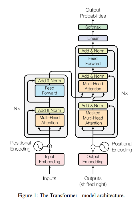
   RNN 考虑了输入时序的问题，而注意力机制是并行输入，不存在时许问题，不融入位置关系就会导致，比如 我 爱 你， 我 你 爱， 爱 我 你 等不同顺序输入后输出相同的结果。
3. VIT 与 Transformer 结构有何不同
   Transformer 中在多头注意力以及前馈神经网络之后做 LN， 而 VIT 是在之前做 LN

• 整体思路

二、模型详解

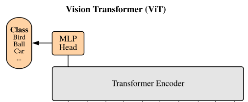
• 模型由三个模块组成：

  1. Linear Projection of Flattened Patches (Embedding层)
  2. Transformer Encoder (图右侧有给出更加详细的结构)
  3. MLP Head（最终用于分类的层结构）

• Embedding 层结构详解

  对于标准的 Transformer 模块，要求输入的是 token（向量）序列，即二维矩阵 [num_token, token_dim]，如下图，token0-9 对应的都是向量，以 ViT-B/16 为例，每个 token 向量长度为 768。
  
  对于图像数据而言，其数据格式为 [H, W, C] 是三维矩阵明显不是 Transformer 想要的。所以需要先通过一个Embedding 层来对数据做个变换。如下图所示，首先将一张图片按给定大小分成一堆 Patches。以 ViT-B/16 为例，将输入图片 (224x224) 按照 16x16 大小的 Patch 进行划分，划分后会得到 ( 224 / 16 ) ² = 196 个 Patches。接着通过线性映射将每个 Patch 映射到一维向量中，以 ViT-B/16 为例，每个 Patche 数据 shape 为 [16, 16, 3] 通过映射得到一个长度为 768 的向量（后面都直接称为 token ）。[16, 16, 3] -> [768]

  在代码实现中，直接通过一个卷积层来实现。 以 ViT-B/16 为例，直接使用一个卷积核大小为 16x16，步距为 16，卷积核个数为 768 的卷积来实现。通过卷积 [224, 224, 3] -> [14, 14, 768]，然后把 H 以及 W 两个维度展平即可 [14, 14, 768] -> [196, 768]，此时正好变成了一个二维矩阵，正是 Transformer 想要的。

  在输入 Transformer Encoder 之前注意需要加上 [class] token 以及 Position Embedding。 在原论文中，作者说参考 BERT，在刚刚得到的一堆 tokens 中插入一个专门用于分类的 [class] token，这个 [class] token 是一个可训练的参数，数据格式和其他 token 一样都是一个向量，以 ViT-B/16 为例，就是一个长度为 768 的向量，与之前从图片中生成的 tokens 拼接在一起，Cat([1, 768], [196, 768]) -> [197, 768]。然后关于 Position Embedding 就是之前 Transformer 中讲到的 Positional Encoding，这里的 Position Embedding 采用的是一个可训练的参数（1D Pos. Emb.），是直接叠加在 tokens 上的（add），所以 shape 要一样。以 ViT-B/16 为例，刚刚拼接 [class] token 后 shape 是 [197, 768]，那么这里的 Position Embedding 的 shape 也是 [197, 768]。
  
  对于 Position Embedding 作者也有做一系列对比试验，在源码中默认使用的是1D Pos. Emb.，对比不使用 Position Embedding 准确率提升了大概 3 个点，和 2D Pos. Emb. 比起来没太大差别。
  

Patch 代码实现

class PatchEmbed(nn.Module):
    """
    2D Image to Patch Embedding
    """
    def __init__(self, img_size=224, patch_size=16, in_c=3, embed_dim=768, norm_layer=None):
        super().__init__()
        img_size = (img_size, img_size) # 224 × 224
        patch_size = (patch_size, patch_size) # 16 × 16
        self.img_size = img_size
        self.patch_size = patch_size
        self.grid_size = (img_size[0] // patch_size[0], img_size[1] // patch_size[1]) # （14 × 14）
        self.num_patches = self.grid_size[0] * self.grid_size[1] # 196

        self.proj = nn.Conv2d(in_c, embed_dim, kernel_size=patch_size, stride=patch_size) # 3，768（卷积核个数），核大小为 16 × 16，步幅 16 -> B × 14 × 14 × 768
        self.norm = norm_layer(embed_dim) if norm_layer else nn.Identity() # 判断是否进行 LN ，Identity:不执行

    def forward(self, x):
        B, C, H, W = x.shape #（B， 3， 224， 224）
        assert H == self.img_size[0] and W == self.img_size[1], \
            f"Input image size ({H}*{W}) doesn't match model ({self.img_size[0]}*{self.img_size[1]})."

        # flatten: [B, C, H, W] -> [B, C, HW]
        # transpose: [B, C, HW] -> [B, HW, C] （）
        x = self.proj(x).flatten(2).transpose(1, 2) # B × 14 × 14 × 768 -> B × 196 × 768
        x = self.norm(x)
        return x
1
2
3
4
5
6
7
8
9
10
11
12
13
14
15
16
17
18
19
20
21
22
23
24
25
26

• Transformer Encoder详解

  Transformer Encoder 其实就是重复堆叠 Encoder Block L 次，下图是 [1] 作者绘制的Encoder Block，主要由以下几部分组成：

  • Layer Norm，这种 Normalization 方法主要是针对 NLP 领域提出的，这里是对每个 token 进行 Norm 处理，之前也有讲过 Layer Norm 不懂的可以参考链接
  • Multi-Head Attention，这个结构之前在讲 Transformer 中很详细的讲过，不在赘述，不了解的可以参考链接
  • Dropout/DropPath，在原论文的代码中是直接使用的 Dropout 层，在但rwightman 实现的代码中使用的是 DropPath（stochastic depth），可能后者会更好一点。
  • MLP Block，如图右侧所示，就是 全连接 + GELU 激活函数 + Dropout 组成也非常简单，需要注意的是第一个全连接层会把输入节点个数翻 4 倍 [197, 768] -> [197, 3072]，第二个全连接层会还原回原节点个数 [197, 3072] -> [197, 768]

Attention 代码实现

class Attention(nn.Module):
    def __init__(self,
                 dim,   # 输入token的dim
                 num_heads=8,
                 qkv_bias=False,
                 qk_scale=None,
                 attn_drop_ratio=0.,
                 proj_drop_ratio=0.):
        super(Attention, self).__init__()
        self.num_heads = num_heads # 8
        head_dim = dim // num_heads # 96
        self.scale = qk_scale or head_dim ** -0.5 # 特征缩放
        self.qkv = nn.Linear(dim, dim * 3, bias=qkv_bias) # 3 × dim 的维度一次产生 Q K V 的三个权重矩阵
        self.attn_drop = nn.Dropout(attn_drop_ratio)
        self.proj = nn.Linear(dim, dim)
        self.proj_drop = nn.Dropout(proj_drop_ratio)

    def forward(self, x):
        # [batch_size, num_patches + 1, total_embed_dim]
        B, N, C = x.shape # [B, 197, 768]

        # qkv(): -> [batch_size, num_patches + 1, 3 * total_embed_dim] -> [B, 197, 3 * 768]
        # reshape: -> [batch_size, num_patches + 1, 3, num_heads, embed_dim_per_head] -> [B, 197, 3 , 8, 288]
        # permute: -> [3, batch_size, num_heads, num_patches + 1, embed_dim_per_head] -> [3, B, 8, 197, 288]
        qkv = self.qkv(x).reshape(B, N, 3, self.num_heads, C // self.num_heads).permute(2, 0, 3, 1, 4)
        # [batch_size, num_heads, num_patches + 1, embed_dim_per_head]
        q, k, v = qkv[0], qkv[1], qkv[2]  # make torchscript happy (cannot use tensor as tuple) [B, 8, 197, 288]

        # transpose: -> [batch_size, num_heads, embed_dim_per_head, num_patches + 1]
        # @: multiply -> [batch_size, num_heads, num_patches + 1, num_patches + 1]
        attn = (q @ k.transpose(-2, -1)) * self.scale # Q * k^T 再放缩
        attn = attn.softmax(dim=-1)
        attn = self.attn_drop(attn)

        # @: multiply -> [batch_size, num_heads, num_patches + 1, embed_dim_per_head]
        # transpose: -> [batch_size, num_patches + 1, num_heads, embed_dim_per_head]
        # reshape: -> [batch_size, num_patches + 1, total_embed_dim]
        x = (attn @ v).transpose(1, 2).reshape(B, N, C) # 转置后和并最后两个维度
        x = self.proj(x) # 连接线性层 [B, 197, 768]
        x = self.proj_drop(x)
        return x
1
2
3
4
5
6
7
8
9
10
11
12
13
14
15
16
17
18
19
20
21
22
23
24
25
26
27
28
29
30
31
32
33
34
35
36
37
38
39
40
41

图中的 Encoder block 代码实现

class Block(nn.Module):
    def __init__(self,
                 dim,
                 num_heads,
                 mlp_ratio=4.,
                 qkv_bias=False,
                 qk_scale=None,
                 drop_ratio=0.,
                 attn_drop_ratio=0.,
                 drop_path_ratio=0.,
                 act_layer=nn.GELU,
                 norm_layer=nn.LayerNorm):
        super(Block, self).__init__()
        self.norm1 = norm_layer(dim) #
        self.attn = Attention(dim, num_heads=num_heads, qkv_bias=qkv_bias, qk_scale=qk_scale,
                              attn_drop_ratio=attn_drop_ratio, proj_drop_ratio=drop_ratio)
        # NOTE: drop path for stochastic depth, we shall see if this is better than dropout here
        self.drop_path = DropPath(drop_path_ratio) if drop_path_ratio > 0. else nn.Identity()
        self.norm2 = norm_layer(dim)
        mlp_hidden_dim = int(dim * mlp_ratio)
        self.mlp = Mlp(in_features=dim, hidden_features=mlp_hidden_dim, act_layer=act_layer, drop=drop_ratio)

    def forward(self, x):
        x = x + self.drop_path(self.attn(self.norm1(x))) # 先 LN 再做 注意力，再残差连接
        x = x + self.drop_path(self.mlp(self.norm2(x))) # 然后再做 LN， 前馈， 再残差
        return x
1
2
3
4
5
6
7
8
9
10
11
12
13
14
15
16
17
18
19
20
21
22
23
24
25
26

• MLP Head 详解

  上面通过 Transformer Encoder 后输出的 shape 和输入的 shape 是保持不变的，以 ViT-B/16 为例，输入的是[197, 768] 输出的还是 [197, 768]。注意，在 Transformer Encoder 后其实还有一个 Layer Norm 没有画出来，后面有作者 [1] 画的 ViT 的模型可以看到详细结构。这里只需要分类的信息，所以只需要提取出 [class] token 生成的对应结果就行，即 [197, 768] 中抽取出 [class] token 对应的 [1, 768]。接着我们通过 MLP Head 得到我们最终的分类结果。MLP Head 原论文中说在训练 ImageNet21K 时是由 Linear+tanh 激活函数 + Linear 组成。但是迁移到ImageNet1K 上或者你自己的数据上时，只用一个 Linear 即可。

MLP 代码实现

class Mlp(nn.Module):
    """
    MLP as used in Vision Transformer, MLP-Mixer and related networks
    """
    def __init__(self, in_features, hidden_features=None, out_features=None, act_layer=nn.GELU, drop=0.):
        super().__init__()
        out_features = out_features or in_features
        hidden_features = hidden_features or in_features
        self.fc1 = nn.Linear(in_features, hidden_features) # 第一层
        self.act = act_layer() # 激活函数
        self.fc2 = nn.Linear(hidden_features, out_features) # 第二层
        self.drop = nn.Dropout(drop)

    def forward(self, x):
        x = self.fc1(x)
        x = self.act(x)
        x = self.drop(x)
        x = self.fc2(x)
        x = self.drop(x)
        return x
1
2
3
4
5
6
7
8
9
10
11
12
13
14
15
16
17
18
19
20

综上处理后 Vision Transformer 代码实现

class VisionTransformer(nn.Module):
    def __init__(self, img_size=224, patch_size=16, in_c=3, num_classes=1000,
                 embed_dim=768, depth=12, num_heads=12, mlp_ratio=4.0, qkv_bias=True,
                 qk_scale=None, representation_size=None, distilled=False, drop_ratio=0.,
                 attn_drop_ratio=0., drop_path_ratio=0., embed_layer=PatchEmbed, norm_layer=None,
                 act_layer=None):
        """
        Args:
            img_size (int, tuple): input image size
            patch_size (int, tuple): patch size
            in_c (int): number of input channels
            num_classes (int): number of classes for classification head
            embed_dim (int): embedding dimension
            depth (int): depth of transformer
            num_heads (int): number of attention heads
            mlp_ratio (int): ratio of mlp hidden dim to embedding dim
            qkv_bias (bool): enable bias for qkv if True
            qk_scale (float): override default qk scale of head_dim ** -0.5 if set
            representation_size (Optional[int]): enable and set representation layer (pre-logits) to this value if set
            distilled (bool): model includes a distillation token and head as in DeiT models
            drop_ratio (float): dropout rate
            attn_drop_ratio (float): attention dropout rate
            drop_path_ratio (float): stochastic depth rate
            embed_layer (nn.Module): patch embedding layer
            norm_layer: (nn.Module): normalization layer
        """
        super(VisionTransformer, self).__init__()
        self.num_classes = num_classes # 分类类别
        self.num_features = self.embed_dim = embed_dim  # 768
        self.num_tokens = 2 if distilled else 1 # 1
        norm_layer = norm_layer or partial(nn.LayerNorm, eps=1e-6)  # LN
        act_layer = act_layer or nn.GELU

        self.patch_embed = embed_layer(img_size=img_size, patch_size=patch_size, in_c=in_c, embed_dim=embed_dim) # PatchEmbed 类构建[B, 196, 768]
        num_patches = self.patch_embed.num_patches

        self.cls_token = nn.Parameter(torch.zeros(1, 1, embed_dim)) # 构建 [B, 1, 768] 的可训练参数
        self.dist_token = nn.Parameter(torch.zeros(1, 1, embed_dim)) if distilled else None
        self.pos_embed = nn.Parameter(torch.zeros(1, num_patches + self.num_tokens, embed_dim)) # [B, 197, 768]，与前面进行对应
        self.pos_drop = nn.Dropout(p=drop_ratio)

        dpr = [x.item() for x in torch.linspace(0, drop_path_ratio, depth)]  # stochastic depth decay rule


        self.blocks = nn.Sequential(*[
            Block(dim=embed_dim, num_heads=num_heads, mlp_ratio=mlp_ratio, qkv_bias=qkv_bias, qk_scale=qk_scale,
                  drop_ratio=drop_ratio, attn_drop_ratio=attn_drop_ratio, drop_path_ratio=dpr[i],
                  norm_layer=norm_layer, act_layer=act_layer)
            for i in range(depth)
        ]) # depth ： 对 blocks 进行堆叠


        self.norm = norm_layer(embed_dim)

        # Representation layer # 这步不用管
        if representation_size and not distilled:
            self.has_logits = True
            self.num_features = representation_size
            self.pre_logits = nn.Sequential(OrderedDict([
                ("fc", nn.Linear(embed_dim, representation_size)),
                ("act", nn.Tanh())
            ]))
        else:
            self.has_logits = False
            self.pre_logits = nn.Identity()

        # Classifier head(s)
        self.head = nn.Linear(self.num_features, num_classes) if num_classes > 0 else nn.Identity()
        self.head_dist = None
        if distilled:
            self.head_dist = nn.Linear(self.embed_dim, self.num_classes) if num_classes > 0 else nn.Identity()

        # Weight init
        nn.init.trunc_normal_(self.pos_embed, std=0.02)
        if self.dist_token is not None:
            nn.init.trunc_normal_(self.dist_token, std=0.02)

        nn.init.trunc_normal_(self.cls_token, std=0.02)
        self.apply(_init_vit_weights)

    def forward_features(self, x):
        # [B, C, H, W] -> [B, num_patches, embed_dim]
        x = self.patch_embed(x)  # [B, 196, 768]
        # [1, 1, 768] -> [B, 1, 768]
        cls_token = self.cls_token.expand(x.shape[0], -1, -1) # 复制 B 份
        if self.dist_token is None:
            x = torch.cat((cls_token, x), dim=1)  # [B, 197, 768]
        else:
            x = torch.cat((cls_token, self.dist_token.expand(x.shape[0], -1, -1), x), dim=1)

        x = self.pos_drop(x + self.pos_embed) # self.pos_embed 位置编码 与 x 相加 [B, 197, 768]
        x = self.blocks(x)  # [B, 197, 768]
        x = self.norm(x) # [B, 197, 768]
        if self.dist_token is None:
            return self.pre_logits(x[:, 0]) # x[:, 0] 切片提取前面部分
        else:
            return x[:, 0], x[:, 1]

    def forward(self, x):
        x = self.forward_features(x) # 提取到 CLS 后
        if self.head_dist is not None:
            x, x_dist = self.head(x[0]), self.head_dist(x[1])
            if self.training and not torch.jit.is_scripting():
                # during inference, return the average of both classifier predictions
                return x, x_dist
            else:
                return (x + x_dist) / 2
        else:
            x = self.head(x) # 全连接得到多分类的输出
        return x
1
2
3
4
5
6
7
8
9
10
11
12
13
14
15
16
17
18
19
20
21
22
23
24
25
26
27
28
29
30
31
32
33
34
35
36
37
38
39
40
41
42
43
44
45
46
47
48
49
50
51
52
53
54
55
56
57
58
59
60
61
62
63
64
65
66
67
68
69
70
71
72
73
74
75
76
77
78
79
80
81
82
83
84
85
86
87
88
89
90
91
92
93
94
95
96
97
98
99
100
101
102
103
104
105
106
107
108
109
110

Vision Transformer 网络结构细节回顾

Reference

[1] Vision Transformer 详解
[2] Vision Transformer（ViT）PyTorch代码全解析（附图解）