-
Show Me the Code之MXNet网络模型(三)
LeNet 是1986年发表的模型。
网络模型
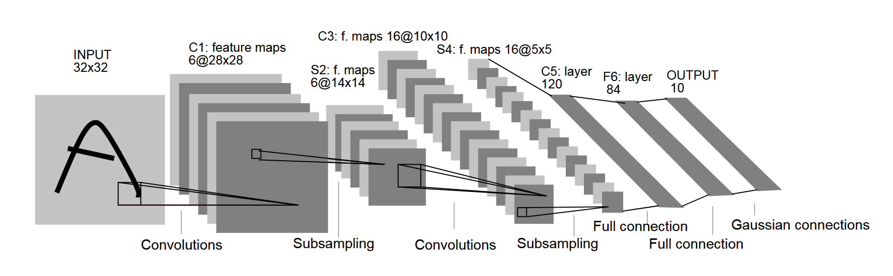
网络层 网络类型 输出数据类型 训练参数 前一层 Input 1x28x28 1-Conv2D 卷积层 6x28x28 6x(1x5x5+1)=156 Input 1-Activation 激活层 6x28x28 1-Conv2D 1-MaxPool2D 池化层 6x14x14 1-Activation 2-Conv2D 卷积层 16x10x10 16x(6x5x5+1)=2416 1-MaxPool2D 2-Activation 激活层 16x10x10 2-Conv2D 2-MaxPool2D 池化层 16x5x5 2-Activation 3-Dense 全连接 120 120x(16x5x5+1)=48120 2-MaxPool2D 3-Activation 激活层 120 3-Dense 4-Dense 全连接 84 84x(120+1)=10164 3-Activation 4-Activation 激活层 84 4-Dense 5-Dense 全连接 10 10x(84+1)=850 4-Activation 统计 61706 由于全连接层占用了绝大部分的训练参数(95.83%),而卷积层比全连接层更加消耗计算力。因此,有人说 “ 全连接层负责参数部分,卷积层负责计算部分 ”。
Show me the code!
说明一下,这里的实现和原本LeNet并不一样。原版的激活函数选的是Sigmoid,而池化为平均值池化。
MXNet 1.5.1
# -*- coding: utf-8 -*- import logging import struct import gzip import numpy as np import mxnet as mx logging.getLogger().setLevel(logging.DEBUG) # 批大小 batch_size = 32 # 学习轮数 train_epoch = 20 # 样本路径 resource_path = "fashion-mnist/" ''' ************************************************************ * 数据准备 ************************************************************ ''' # 定义读取数据的函数 def read_data( label_url, image_url ): with gzip.open( label_url ) as flbl: # 读入标签文件头 magic, num = struct.unpack(">II", flbl.read(8)) # 读入标签内容 label = np.frombuffer( flbl.read(), dtype = np.uint8 ) with gzip.open( image_url, 'rb' ) as fimg: # 读入图像文件头,rows和cols都是28 magic, num, rows, cols = struct.unpack( ">IIII", fimg.read(16) ) # 读入图像内容 image = np.frombuffer( fimg.read(), dtype = np.uint8 ) # 设置为正确的数组格式 image = image.reshape( len(label), 1, rows, cols ) # 归一化到 0~1 image = image.astype( np.float32 ) / 255.0 return (label, image) # 读入数据 # 注意路径的问题 ( train_lbl, train_img ) = read_data( resource_path + 'train-labels-idx1-ubyte.gz', resource_path + 'train-images-idx3-ubyte.gz' ) ( eval_lbl , eval_img ) = read_data( resource_path + 't10k-labels-idx1-ubyte.gz', resource_path + 't10k-images-idx3-ubyte.gz' ) # 迭代器 train_iter = mx.io.NDArrayIter( train_img, train_lbl, batch_size, shuffle=True ) eval_iter = mx.io.NDArrayIter( eval_img , eval_lbl , batch_size ) # 验证集可以省略shuffle ''' ************************************************************ * 定义神经网络模型 ************************************************************ ''' # 输入层 net = mx.sym.var( 'data' ) # 第1层隐藏层 net = mx.sym.Convolution (data=net, name='layer1_conv', num_filter=6, kernel=(5,5), pad=(2,2)) net = mx.sym.Activation (data=net, name='layer1_act' , act_type='relu') net = mx.sym.Pooling (data=net, name='layer1_pool', kernel=(2,2), stride=(2,2), pool_type='max') # 第2层隐藏层 net = mx.sym.Convolution (data=net, name='layer2_conv', num_filter=16, kernel=(5,5)) net = mx.sym.Activation (data=net, name='layer2_act' , act_type='relu') net = mx.sym.Pooling (data=net, name='layer2_pool', kernel=(2,2), stride=(2,2), pool_type='max') # 第3层隐藏层 net = mx.sym.Flatten (data=net, name='flatten') # 将图像摊平 net = mx.sym.FullyConnected(data=net, name='layer3_fc' , num_hidden=120) net = mx.sym.Activation (data=net, name='layer3_act' , act_type='relu') # 第4层隐藏层 net = mx.sym.FullyConnected(data=net, name='layer4_fc' , num_hidden=84) net = mx.sym.Activation (data=net, name='layer4_act' , act_type='relu') # 输出层 net = mx.sym.FullyConnected(data=net, name='layer5_fc' , num_hidden=10) net = mx.sym.SoftmaxOutput (data=net, name='softmax') # Softmax也是激活层 # 网络模型 ctx = mx.gpu() if mx.test_utils.list_gpus() else mx.cpu() # 有GPU就用GPU module = mx.mod.Module(symbol=net, context=ctx) # 网络模型可视化 # shape = {'data':(batch_size, 1, 28, 28)} # mx.viz.print_summary(symbol=net, shape=shape) # mx.viz.plot_network(symbol=net, shape=shape).view() ''' ************************************************************ * 训练神经网络 ************************************************************ ''' # 定义评价标准(Evaluation Metric) eval_metrics = mx.metric.CompositeEvalMetric() eval_metrics.add( mx.metric.Accuracy() ); # 准确率 eval_metrics.add( mx.metric.CrossEntropy() ); # 交叉熵 print("start train...") module.fit( train_data = train_iter, # 训练集 eval_data = eval_iter, # 验证集 eval_metric = eval_metrics, # 评价标准 num_epoch = train_epoch, # 训练轮数 initializer = mx.initializer.Xavier(), # Xavier初始化策略 optimizer = 'sgd', # 随机梯度下降算法 optimizer_params = { 'learning_rate': 0.01, # 学习率 'momentum': 0.9 # 惯性动量 } )- 1
- 2
- 3
- 4
- 5
- 6
- 7
- 8
- 9
- 10
- 11
- 12
- 13
- 14
- 15
- 16
- 17
- 18
- 19
- 20
- 21
- 22
- 23
- 24
- 25
- 26
- 27
- 28
- 29
- 30
- 31
- 32
- 33
- 34
- 35
- 36
- 37
- 38
- 39
- 40
- 41
- 42
- 43
- 44
- 45
- 46
- 47
- 48
- 49
- 50
- 51
- 52
- 53
- 54
- 55
- 56
- 57
- 58
- 59
- 60
- 61
- 62
- 63
- 64
- 65
- 66
- 67
- 68
- 69
- 70
- 71
- 72
- 73
- 74
- 75
- 76
- 77
- 78
- 79
- 80
- 81
- 82
- 83
- 84
- 85
- 86
- 87
- 88
- 89
- 90
- 91
- 92
- 93
- 94
- 95
- 96
- 97
- 98
- 99
- 100
- 101
- 102
- 103
- 104
- 105
- 106
- 107
- 108
- 109
- 110
- 111
- 112
- 113
- 114
INFO:root:Epoch[0] Train-accuracy=0.791900
INFO:root:Epoch[0] Train-cross-entropy=0.560617
INFO:root:Epoch[0] Time cost=5.205
INFO:root:Epoch[0] Validation-accuracy=0.860024
INFO:root:Epoch[0] Validation-cross-entropy=0.387932
INFO:root:Epoch[1] Train-accuracy=0.871650
INFO:root:Epoch[1] Train-cross-entropy=0.351662
INFO:root:Epoch[1] Time cost=5.167
INFO:root:Epoch[1] Validation-accuracy=0.883786
INFO:root:Epoch[1] Validation-cross-entropy=0.316452
…
INFO:root:Epoch[19] Train-accuracy=0.942633
INFO:root:Epoch[19] Train-cross-entropy=0.151282
INFO:root:Epoch[19] Time cost=5.186
INFO:root:Epoch[19] Validation-accuracy=0.907548
INFO:root:Epoch[19] Validation-cross-entropy=0.307947MXNet 1.9.1
上面的代码,到了MXNet 1.6.0版本就用不了了。
下面是新的实现。import time import struct import gzip import numpy as np import matplotlib.pyplot as plt import mxnet as mx- 1
- 2
- 3
- 4
- 5
- 6
设置批大小和CPU
batch_size = 32 device = mx.cpu(0)- 1
- 2
定义功能函数,读取图片
def read_data( label_url, image_url ): with gzip.open( label_url ) as flbl: # 读入标签文件头 magic, num = struct.unpack( ">II", flbl.read(8) ) label = np.frombuffer( flbl.read(), dtype = np.uint8 ) with gzip.open( image_url, 'rb' ) as fimg: # 读入图像文件头,rows和cols都是28 magic, num, rows, cols = struct.unpack( ">IIII", fimg.read(16) ) # 读入图像内容 image = np.frombuffer( fimg.read(), dtype = np.uint8 ) # 设置为正确的数组格式 image = image.reshape( num, 1, rows, cols ) # 归一化到 [-1,1] image = image.astype( np.float32 ) / 255.0 return (label, image)- 1
- 2
- 3
- 4
- 5
- 6
- 7
- 8
- 9
- 10
- 11
- 12
- 13
- 14
- 15
读取数据,打印维度
( train_lbl, train_img ) = read_data( 'fashion-mnist/train-labels-idx1-ubyte.gz', 'fashion-mnist/train-images-idx3-ubyte.gz' ) ( eval_lbl , eval_img ) = read_data( 'fashion-mnist/t10k-labels-idx1-ubyte.gz', 'fashion-mnist/t10k-images-idx3-ubyte.gz' ) print("train:", type(train_img), train_img.shape, train_img.dtype) print("eval: ", type(eval_img), eval_img.shape, eval_img.dtype )- 1
- 2
- 3
- 4
- 5
- 6
- 7
- 8
- 9
- 10
train: <class ‘numpy.ndarray’> (60000, 1, 28, 28) float32
eval: <class ‘numpy.ndarray’> (10000, 1, 28, 28) float32查看数据图片
texts = ( 't-shirt', 'trouser', 'pullover', 'dress', 'coat', 'sandal', 'shirt', 'sneaker', 'bag', 'ankle boot' ) idxs = (0, 1, 2, 3, 4, 5, 7, 9, 14, 21) for i in range(10): plt.subplot(2, 5, i + 1) idx = idxs[i] plt.xticks([]) plt.yticks([]) plt.title(texts[train_lbl[idx]]) img = train_img[idx][0].astype( np.float32 ) plt.imshow(img, interpolation='none', cmap='Blues') plt.show()- 1
- 2
- 3
- 4
- 5
- 6
- 7
- 8
- 9
- 10
- 11
- 12
- 13
- 14
- 15
- 16

创建训练迭代器。这一步设置了批大小和训练集的随机排序。train_data = mx.gluon.data.DataLoader( mx.gluon.data.ArrayDataset(train_img, train_lbl), batch_size=batch_size, shuffle=True ) eval_data = mx.gluon.data.DataLoader( mx.gluon.data.ArrayDataset(eval_img, eval_lbl), batch_size=batch_size, shuffle=False )- 1
- 2
- 3
- 4
- 5
- 6
- 7
- 8
- 9
- 10
定义一个评价类。用MXNet自带的也行,但是我想封装show()
class UserMetrics(mx.metric.CompositeEvalMetric): def __init__(self, name='user', output_names=None, label_names=None): # 初始化PyTorch父类 super().__init__(name=name, output_names=output_names, label_names=label_names) super().add( mx.metric.Accuracy() ) super().add( mx.metric.CrossEntropy() ) def reset(self): super().reset() self.tic = time.time() def show(self, epoch=0, tag='[ ]'): cost = time.time() - self.tic name, val = super().get() print("Epoch %2d: %s cost:%.1fs %s:%.3f, %s:%.3f" % ( epoch, tag, cost, name[0], val[0], name[1], val[1] ) )- 1
- 2
- 3
- 4
- 5
- 6
- 7
- 8
- 9
- 10
- 11
- 12
- 13
- 14
- 15
定义网络
# 网络类型 net = mx.gluon.nn.HybridSequential() # 中间层 net.add( # 第一层 mx.gluon.nn.Conv2D( channels=6, kernel_size=(5,5), strides=(1,1), padding=(2,2) ), mx.gluon.nn.Activation( 'relu' ), mx.gluon.nn.MaxPool2D( pool_size=(2,2) ), # 第二层 mx.gluon.nn.Conv2D( channels=16, kernel_size=(5,5), strides=(1,1), padding=(0,0) ), mx.gluon.nn.Activation( 'relu' ), mx.gluon.nn.MaxPool2D( pool_size=(2,2) ), # 第三层 mx.gluon.nn.Dense( 120 ), mx.gluon.nn.Activation( 'relu' ), # 第四层 mx.gluon.nn.Dense( 84 ), mx.gluon.nn.Activation( 'relu' ) ) # 输出层 net.output = mx.gluon.nn.Dense( 10 ) # 初始化 net.initialize( init=mx.init.Xavier(), ctx=device ) # 展示网络 net.summary(mx.ndarray.zeros(shape=(1, 1, 28, 28), dtype=np.float32, ctx=device)) # 符号式加速 net.hybridize()- 1
- 2
- 3
- 4
- 5
- 6
- 7
- 8
- 9
- 10
- 11
- 12
- 13
- 14
- 15
- 16
- 17
- 18
- 19
- 20
- 21
- 22
- 23
- 24
- 25
- 26
- 27
- 28
- 29
- 30
- 31
- 32

损失函数,训练器,评价器
# 损失函数 loss_function = mx.gluon.loss.SoftmaxCrossEntropyLoss() # 求解器 optimizer = mx.optimizer.SGD( learning_rate=0.01, momentum=0.0, multi_precision=False ) # 训练器 trainer = mx.gluon.Trainer( params=net.collect_params(), optimizer=optimizer ) # 评价器 metrics = UserMetrics()- 1
- 2
- 3
- 4
- 5
- 6
- 7
- 8
开始训练 20 epoch
for epoch in range(20): # train metrics.reset() for datas, labels in train_data: actual_batch_size = datas.shape[0] # split batch and load into corresponding devices datas = mx.gluon.utils.split_and_load( datas, [device] ) labels = mx.gluon.utils.split_and_load( labels, [device] ) # The forward pass and the loss computation with mx.autograd.record(): outputs = [ net(data) for data in datas ] losses = [ loss_function(output, label) for output, label in zip(outputs, labels) ] # compute gradients for loss in losses: loss.backward() # update parameters trainer.step( batch_size=actual_batch_size ) # update metric for output, label in zip(outputs, labels): metrics.update( preds=mx.ndarray.softmax(output, axis=1), labels=label ) metrics.show( epoch=epoch, tag='[ train ]' ) # eval metrics.reset() for datas, labels in eval_data: # split batch and load into corresponding devices datas = mx.gluon.utils.split_and_load(datas, [device]) labels = mx.gluon.utils.split_and_load(labels, [device]) # The forward pass outputs = [ net(data) for data in datas ] # update metric for output, label in zip(outputs, labels): metrics.update( preds=mx.ndarray.softmax(output, axis=1), labels=label ) metrics.show( epoch=epoch, tag='[ eval ]' )- 1
- 2
- 3
- 4
- 5
- 6
- 7
- 8
- 9
- 10
- 11
- 12
- 13
- 14
- 15
- 16
- 17
- 18
- 19
- 20
- 21
- 22
- 23
- 24
- 25
- 26
- 27
- 28
- 29
- 30
- 31
- 32
- 33
- 34
- 35
- 36
- 37
- 38
- 39
- 40
- 41
Epoch 0: [ train ] cost:8.0s accuracy:0.693, cross-entropy:0.847
Epoch 0: [ eval ] cost:0.6s accuracy:0.784, cross-entropy:0.588
Epoch 1: [ train ] cost:7.9s accuracy:0.805, cross-entropy:0.531
Epoch 1: [ eval ] cost:0.6s accuracy:0.837, cross-entropy:0.453
Epoch 2: [ train ] cost:7.9s accuracy:0.835, cross-entropy:0.452
Epoch 2: [ eval ] cost:0.6s accuracy:0.851, cross-entropy:0.420
…
Epoch 18: [ train ] cost:8.0s accuracy:0.908, cross-entropy:0.250
Epoch 18: [ eval ] cost:0.6s accuracy:0.896, cross-entropy:0.290
Epoch 19: [ train ] cost:8.0s accuracy:0.910, cross-entropy:0.244
Epoch 19: [ eval ] cost:0.6s accuracy:0.899, cross-entropy:0.273 -
相关阅读:
SpringMVC源码分析(三)HandlerExceptionResolver启动和异常处理源码分析
openGauss学习笔记-241 openGauss性能调优-SQL调优-审视和修改表定义
十、pygame小游戏开发
用Java实现Nginx插件
使用Cpolar+freekan源码 创建在线视频网站
MySQL的MHA
MySQL——数据的增删改
k8s /apis/batch/v1beta1 /apis/policy/v1beta1 接口作用
嫌学校软件太烂,父母做了开源APP,却被官方报警
EfficientNeRF阅读笔记
- 原文地址:https://blog.csdn.net/tissar/article/details/86644945
